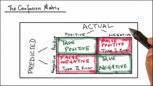
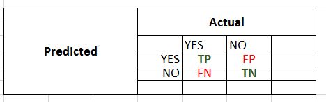
Confusion Matrix
Label - Disease
Binary Values - YES, NO
TP = True Positives - YES classified as YES
TN = True Negatives - NO classified as NO
FP = False Positive - NO classified as YES
FN = False Negative - YES classified as NO
Predicted Positives
First Row Total = TP + FP
Actual Positives
First Column Total = TP + FN
Predicted Negatives
Second Row Total = TN + FN
Actual Negatives
Second Column Total = TN + FP
Prediction Measures
Predictions are correct when the predicted values match the actual values of the test dataset label. The diagonal values in the confusion matrix are the matching values and hence indicate the correct predictions.
The non-diagonal values of the confusion matrix are the mis-match between actual and predicted values of the test dataset label; and hence indicate the mis-classifications.
Correct Predictions:
True Positives (TP)
The trained model predicts the patient has the disease and the patient actually has the disease. That is predicted values 'YES' for the label 'disease' match with the actual values 'YES' of the test data.
True Negatives (TN)
The trained model predicts the patient does not have the disease and the patient is actually disease free. That is predicted values 'NO' for the label 'disease' match with the actual values 'NO' of the test data.
Mis-classifications:
False Positives (FP) - Type I error
The trained model predicts the patient has the disease but the patient is actually disease free. That is predicted values 'YES' for the label 'disease' do-not-match with the actual values 'NO' of the test data.
This is also known as Type I error wrt the null hypothesis.
False Negative (FN) - Type II error
The trained model predicts the patient does not have the disease but the patient actually has the disease. That is predicted values 'NO' for the label 'disease' do-not-match with the actual values 'YES' of the test data.
This is also known as Type II error wrt the null hypothesis.
Based on these four values of the confusion matrix below metrics are used to measure the predictive power of the binary classifiers:
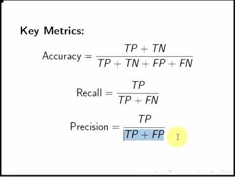
Accuracy: Correct Predictions on Total
Proportion of correct classifications overall. That is total correct predictions over total observations?

Error Rate: Incorrect Predictions on Total
Proportion of incorrect predictions overall? That is total incorrect predictions over total observations.
Error = 1 - Accuracy

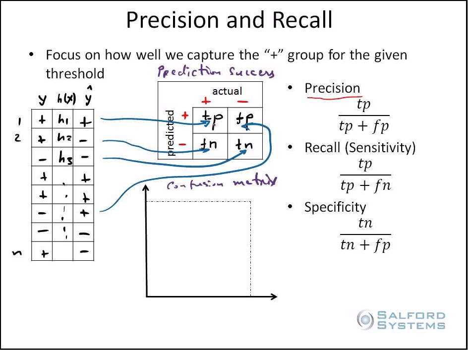
Precision: Correct Positive Predictions over Total Positive Predictions
How many of the 'YES' predictions are correct from the total 'YES' predictions?

Recall (Sensitivity): Correct Positive Predictions over Actual Positive Values
How many of the 'YES' predictions are correct from the actual 'YES' values (i.e. columns total)?

Specificity: Correct Negative Predictions over Actual Negative Values
How many of the 'NO' predictions are correct from the actual 'NO' values (i.e. second column total)?

Binary Classification Example
We classify the sale of child car seats as high or low and use confusion matrix to calculate the accuracy, precision, recall and specificity of the model.
Understanding the Carseats dataset
We will use Carseats dataset from ILSR library.
The binary classification problem is to predict the Sales as high or low using remaining 10 variables as predictors for the classifier.
# see description of Carseats dataset
?Carseats
# Carseats {ISLR} R Documentation
# Sales of Child Car Seats
# Description
# A simulated data set containing sales of child car seats at 400 different stores.
# A data frame with 400 observations on the 11 variables.
# check dimensions of data set
dim(Carseats)
#[1] 400 11
names(Carseats)
# [1] "Sales" "CompPrice" "Income" "Advertising"
# [5] "Population" "Price" "ShelveLoc" "Age"
# [9] "Education" "Urban" "US"
str(Carseats)
# 'data.frame': 400 obs. of 11 variables:
# $ Sales : num 9.5 11.22 10.06 7.4 4.15 ...
# $ CompPrice : num 138 111 113 117 141 124 115 136 132 132 ...
# $ Income : num 73 48 35 100 64 113 105 81 110 113 ...
# $ Advertising: num 11 16 10 4 3 13 0 15 0 0 ...
# $ Population : num 276 260 269 466 340 501 45 425 108 131 ...
# $ Price : num 120 83 80 97 128 72 108 120 124 124 ...
# $ ShelveLoc : Factor w/ 3 levels "Bad","Good","Medium": 1 2 3 3 1 1 3 2 3 3 ...
# $ Age : num 42 65 59 55 38 78 71 67 76 76 ...
# $ Education : num 17 10 12 14 13 16 15 10 10 17 ...
# $ Urban : Factor w/ 2 levels "No","Yes": 2 2 2 2 2 1 2 2 1 1 ...
# $ US : Factor w/ 2 levels "No","Yes": 2 2 2 2 1 2 1 2 1 2 ...
Set seed
To make result reproducible
set.seed(2)
Fit the tree model
The model is built using training dataset and the predictor depends on all features.
# fit the tree model using training data
tree_model = tree(Sales_High~., training_data)
# use the model to predict test data
test_pred = predict(tree_model, testing_data, type="class")
Calculating Model Prediction Success
Accuracy
Error Rate
Precision
Recall
Specificity
# confusion matrix values
TP = 35
TN = 68
FP = 10
FN = 21
# row and column totals
Pred_Positives = TP + FP
Pred_Positives
#[1] 45
Pred_Negatives = TN + FN
Pred_Negatives
#[1] 89
Actual_Positives = TP + FN
Actual_Positives
# [1] 56
Actual_Negatives = TN + FP
Actual_Negatives
# [1] 78
Total_test_data = TP + TN + FP + FN
Total_test_data
# [1] 134
# Accuracy
Accuracy = (TP + TN)/Total_test_data
Accuracy
#[1] 0.7686567
# Error_rate
Error_rate = (FP + FN)/Total_test_data
Error_rate
# [1] 0.2313433
Error_rate = 1- Accuracy
Error_rate
# [1] 0.2313433
# Precision
Precision = TP/Pred_Positives
Precision
# [1] 0.7777778
# Recall_Sensitivity
Recall_Sensitivity = TP/Actual_Positives
Recall_Sensitivity
# [1] 0.625
# Specificity
Specificity = TN/Actual_Negatives
Specificity
# [1] 0.8717949