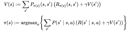
Algorithms to solve MDP
The solution for an MDP is a policy which describes the best action for each state in the MDP, known as the optimal policy. This optimal policy can be found through a variety of methods, like dynamic programming.
Some dynamic programming solutions require knowledge of the state transition function P and the reward function R. Others can solve for the optimal policy of an MDP using experimentation alone.
Consider the case in which state transition function P and reward function R for an MDP is given, and we seek the optimal policy π* that maximizes the expected discounted reward.
The standard family of algorithms to calculate this optimal policy requires storage for two arrays indexed by state: value V, which contains real values, and policy π, which contains actions. At the end of the algorithm, π will contain the solution and V(s) will contain the discounted sum of the rewards to be earned (on average) by following that solution from state s.
The algorithm has two steps:
- a value update and
- a policy update
which are repeated in some order for all the states until no further changes take place. Both recursively update a new estimation of the optimal policy and state value using an older estimation of those values.
Their order depends on the variant of the algorithm; one can also do them for all states at once or state by state, and more often to some states than others. As long as no state is permanently excluded from either of the steps, the algorithm will eventually arrive at the correct solution
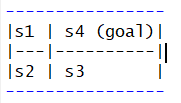
2x2 Grid MDP Problem
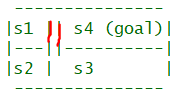
si - indicates the state in grid i
The red boundary indicates the move is not allowed.
s1 to s4 and s4 to s1 moves are NOT allowed
MDP Environment Description
Here an agent is intended to navigate from an arbitrary starting position to a goal position.
The grid is surrounded by a wall, which makes it impossible for the agent to move off the grid. In addition, the agent faces a wall between s1 and s4.
If the agent reaches the goal position, it earns a reward of 10.
Crossing each square of the grid results in a negative reward of -1
Constraints For State-Action
2x2 Grid
When the agent selects an action:
- there is a 70% probability that that action will occur
- there is 20 % probability the agent will stay in the same state
- and there is 10 % probability that the agent will move in a lateral direction to the action selected.
Rewards:
- if agent enter S1 from anywhere reward is -1
- if agent enter S2 from anywhere reward is -1
- if agent enter S3 from anywhere reward is -1
- if agent enter S4 from anywhere reward is 10
MDP Policy Iteration
Based on the above environment information along with state transition probabilities and rewards for the transitions we find a model-based optimal policy for Grid World MDP to reach the goal state for S4.
- Design an MDP that finds the optimal policy to the 2 x 2 grid problem.
- Create individual matrices with pre-specified (random) transition probabilities for each action
{these represent the stochasticity of the randomness of action actually taken to that is selected} - These transition matrices reflect the following randomness of action taken vis a vis action selected.
Probability Transition Matrix
We build the state-action transition matrix based on the model information/constraints we have about the grid MDP environment.
Below is the explanation for transition probability for all the four states S1, S2, S3, S4 for the UP action for illustration - based on which we build the transition matrices in R for remaining actions LEFT, DOWN, RIGHT
S1-UP
0.7 - probability that UP action will occur; in which case it will hit the upper boundary and remain in the same S1
0.2 - probability that agent doesn't take action and prefers to remain in the same state, so ends up in state S1
0.1 - Lateral move would be left or right, in which case it will end up in the same state S1
So (0.7+02+01 = 1 ) probability of S1-UP action resulting in state S1 is 100 %. Therefore, probability of transitioning to other states is 0.
S2-UP
0.7 - probability that it will go UP and result in state S1
0.2 - probability that it will remain in same state S2
0.1 - probability that it will move laterally, left hits boundary, right results in state S3
No other transitions are possible, so probability for resulting in state S4 is zero.
S3-UP
0.7 - probability that action will occur and result in state S4
0.2 - probability that the agent will not take action and remain in the same state S3
0.1 - probability that the agent takes lateral move; right will hit the boundary and left will result in state S2
S4-UP
0.7 - probability that action will occur and result in state S4
0.2 - probability that the agent will not take action and remain in the same state S4
0.1 - probability that agent takes lateral move; right will hit the boundary and left is not allowed so will remain in the same state S4
Similarly, we can build the transition probability matrix for actions LEFT, RIGHT and DOWN.
Probability Matrix for UP action for states S1, S2, S3, S4
To State
State-Action S1 S2 S3 S4
S1-UP (0.7+02+0.1) 0 0 0
S2-UP 0.7 0.2 0.1 0
S3-UP 0 0.1 0.2 0.7
S4-UP 0 0 0 (0.7+0.2+0.1)
Probability Matrix for LEFT action for states S1, S2, S3, S4
To State
State-Action S1 S2 S3 S4
S1-LEFT (0.7+02) 0.1 0 0
S2-LEFT 0.1 (0.7+02) 0 0
S3-LEFT 0 0.7 0.2 0.1
S4-LEFT 0 0 0.1 (0.7+0.2)
Probability Matrix for RIGHT action for states S1, S2, S3, S4
To State
State-Action S1 S2 S3 S4
S1-RIGHT (0.7+02) 0.1 0 0
S2-RIGHT 0.1 0.2 0.7 0
S3-RIGHT 0 0 (0.7+0.2 ) 0.1
S4-RIGHT 0 0 0.1 (0.7+0.2)
Probability Matrix for DOWN action for states S1, S2, S3, S4
To State
State-Action S1 S2 S3 S4
S1-DOWN (0.2 + 0.1) 0.7 0 0
S2-DOWN 0 (0.7 +0.2) 0.1 0
S3-DOWN 0 1 (0.7 +0.2 ) 0
S4-DOWN 0 0 0.7 (0.2+0.1)
Reward Matrix
- if you enter S1 from anywhere you get reward -1
- if you enter S2 from anywhere you get reward -1
- if you enter S3 from anywhere you get reward -1
- if you enter S4 from anywhere you get reward 10
# Create a list T for the transition probabilities
T = list(up = up, left = left, down = down, right = right)
# Create matrix with rewards:
R = matrix(c(-1, -1, -1, -1,
-1, -1, -1, -1,
-1, -1, -1, -1,
10, 10, 10, 10),
nrow = 4, ncol = 4, byrow = TRUE)
Cross check our MDP
We built the transition matrix and reward matrix to design our MDP. Before we go ahead to find the optimal policy for the grid problem we need to check its validity.
We use the mdp_check function.
![]()
# Check if this provides a well-defined MDP
?mdp_check
"
Checks the validity of a MDP
Details
mdp_check checks whether the MDP defined by the transition probability array (P) and the reward matrix (R) is valid.
If P and R are correct, the function returns an empty error message.
In the opposite case, the function returns an error message describing the problem.
Usage
mdp_check(P, R)
Arguments
P
transition probability array.
P can be a 3 dimensions array [S,S,A] or a list [[A]],
each element containing a sparse matrix [S,S].
R
reward array. R can be a 3 dimensions array [S,S,A] or a list [[A]],
each element containing a sparse matrix [S,S] or
a 2 dimensional matrix [S,A] possibly sparse.
"
mdp_check(T, R)
## [1] ""Use Policy Iteration
To find the optimal policy we use the mdp policy iteration method with discount factor 0.9
![]()
# Run policy iteration with discount factor g = 0.9
?mdp_policy_iteration
"
Solves discounted MDP with policy iteration algorithm
Usage
mdp_policy_iteration(P, R, discount, policy0, max_iter, eval_type)
Details
mdp_policy_iteration applies the policy iteration algorithm to solve discounted MDP.
The algorithm consists in improving the policy iteratively, using the evaluation of the current policy. Iterating is stopped when two successive policies are identical or when a specified number (max_iter) of iterations have been performed.
"
m = mdp_policy_iteration(P = T,
R = R,
discount = 0.9)
Conclusion
So the optimal policy is to move down, right, up, up.
It shows that when we take the actions based on optimal policy the cumulative values increases until it reaches one hundred.
Now, let's find the optimal policy using value iteration.
Use Value Iteration
To find the optimal policy we use the mdp value iteration method with discount factor 0.9
![]()
# Run policy iteration with discount factor g = 0.9
?mdp_value_iteration
"
Solves discounted MDP using value iteration algorithm
Description
Solves discounted MDP with value iteration algorithm
Usage
mdp_value_iteration(P, R, discount, epsilon, max_iter, V0)
Arguments
P
transition probability array. P can be a 3 dimensions array [S,S,A] or a list [[A]], each element containing a sparse matrix [S,S].
R
reward array. R can be a 3 dimensions array [S,S,A] or a list [[A]], each element containing a sparse matrix [S,S] or a 2 dimensional matrix [S,A] possibly sparse.
discount
discount factor. discount is a real number which belongs to [0; 1[. For discount equals to 1, a warning recalls to check conditions of convergence.
epsilon
(optional) : search for an epsilon-optimal policy. epsilon is a real in ]0; 1]. By default, epsilon = 0.01.
max_iter
(optional) : maximum number of iterations. max_iter is an integer greater than 0. If the value given in argument is greater than a computed bound, a warning informs that the computed bound will be considered. By default, if discount is not egal to 1, a bound for max_iter is computed, if not max_iter = 1000.
V0
(optional) : starting value function. V0 is a (Sx1) vector. By default, V0 is only composed of 0 elements.
"
mV = mdp_value_iteration(P = T,
R = R,
discount = 0.9)
mdp_value_iteration output
Details:
mdp_value_iteration applies the value iteration algorithm to solve discounted MDP. The algorithm consists in solving Bellman''s equation iteratively. Iterating is stopped when an epsilon-optimal policy is found or after a specified number (max_iter) of iterations.
Value:
policy - optimal policy. policy is a S length vector.
Each element is an integer corresponding to an action which maximizes the value function.
iter - number of done iterations.
cpu_time - CPU time used to run the program.
# Examine the output
mV$policy
# [1] 3 4 1 1
names(T)[mV$policy]
# [1] "down" "right" "up" "up"
mV$V
# [1] 44.74884 55.58281 69.68448 86.49148
mV$iter
# [1] 19
Conclusion
The function grid world simulates the environment for the agent to learn from.
![]()
So the optimal policy using value iteration is same as that using policy iteration. It is to move down, right, up, up.
It shows that when we follow the value iteration cumulative values may NOT reach one hundred until the goal is reached.