Cross Validation of Tree

To improve accuracy

To reduce error rate of a classification tree model 'pruning' can be used. It is a cross-validation technique which gives the size of tree and the corresponding deviance or error. Using the size that has the lowest deviance we can build the tree model for that size and improve accuracy.

cv-tree-without-pruning

cv-error-vs-size

cv-tree-after-pruning

Programming Logic

Steps to fit classification tree model for prediction, do cross validation to check accuracy and use 'pruning' to reduce error of the classification tree prediction model.

Pre-requisite:

Understand the data set for pre-processing that may be requierd to create sample dataset for training and testing.

Step 1:
Install the required R packages and load them

Step 2:
Set up the environment options, if any
Set seed

Step 3:
Pre-process the data set. Create categorical variable 'High' based on the Sales variable

Step 3:
Create train and test data from data set

Step 4:
Fit the tree model to train data using formula where predictor uses all features

Step 5:
Use tree model to predict target variable on testing data set

Step 6:
Measure the accuracy of predicted values using actual values in test data set

Step 7:
Use cross validation to determine the tree 'size' for which 'dev' i.e. error is lowest

Step 8:
Prune the tree model for the best size per cross validation and predict for the testing data

Step 9:
Compare the accuracy of pruned model with the original for improvement in accuracy of prediction

Install required R packages 

install.packages("ISLR")
install.packages("tree")


Load installed R packages 

libs = c("ISLR","tree")
lapply(libs, require, character.only=TRUE)


Understanding the data set to build prediction model

We will use Carseats dataset from ILSR library.

Target variable 'Sales' is a continuous variable, since we cannot do classification on continuous variable  we create a new variable 'High' to indicate sales is high or not.  We assign categorical values 'Yes' or 'No'  to High based on condition that sales value is greater than the median sales value.

# check dimensions of data set

dim(Carseats)
#[1] 400 11

names(Carseats)
# [1] "Sales" "CompPrice" "Income" "Advertising"
# [5] "Population" "Price" "ShelveLoc" "Age"
# [9] "Education" "Urban" "US"

str(Carseats)

# 'data.frame': 400 obs. of 11 variables:
# $ Sales : num 9.5 11.22 10.06 7.4 4.15 ...
# $ CompPrice : num 138 111 113 117 141 124 115 136 132 132 ...
# $ Income : num 73 48 35 100 64 113 105 81 110 113 ...
# $ Advertising: num 11 16 10 4 3 13 0 15 0 0 ...
# $ Population : num 276 260 269 466 340 501 45 425 108 131 ...
# $ Price : num 120 83 80 97 128 72 108 120 124 124 ...
# $ ShelveLoc : Factor w/ 3 levels "Bad","Good","Medium": 1 2 3 3 1 1 3 2 3 3 ...
# $ Age : num 42 65 59 55 38 78 71 67 76 76 ...
# $ Education : num 17 10 12 14 13 16 15 10 10 17 ...
# $ Urban : Factor w/ 2 levels "No","Yes": 2 2 2 2 2 1 2 2 1 1 ...
# $ US : Factor w/ 2 levels "No","Yes": 2 2 2 2 1 2 1 2 1 2 ...

Pre-processing the data set

In order to decide what indicates high sales we look at the statistics of sales and set a condition based on the range and median value.

# data manipulation to set condition for new variable

range(Carseats$Sales)
#[1] 0.00 16.27

summary(Carseats$Sales)
# Min.     1st Qu.  Median  Mean   3rd Qu.  Max.
# 0.000  5.390    7.490      7.496   9.320     16.270

# create categorical variable to indicate high sales

High = ifelse(Carseats$Sales >= 8, "Yes", "No")

# append High to Carseat dataset
CarSeats_new = data.frame(Carseats, High)

dim(CarSeats_new)
# [1] 400 12

names(CarSeats_new)
# [1] "Sales" "CompPrice" "Income" "Advertising" "Population"
# [6] "Price" "ShelveLoc" "Age" "Education" "Urban"
# [11] "US" "High"

# now we can remove the first column 'Sales'
# we will use categorical variable 'High' instead

CarSeats_new = CarSeats_new[,-1]

dim(CarSeats_new)
# [1] 400 11

names(CarSeats_new)
# [1] "CompPrice" "Income" "Advertising" "Population" "Price"
# [6] "ShelveLoc" "Age" "Education" "Urban" "US"
# [11] "High"

Set seed

To make result reproducible

set.seed(2)

Create train and test data set

Split the data set in to two equal parts for training and testing

Use sample function to generate random numbers equal to half the size of data set, use these random numbers as index to get training data set and the remaining - not these indexes - indicated with minus sign to get testing data set.

# generate random numbers for train index

train = sample(1:nrow(CarSeats_new), nrow(CarSeats_new)/2)

str(train)

# int [1:200] 74 281 229 67 374 373 51 328 184 216 ...

train
# [1] 74 281 229 67 374 373 51 328 184 216 391 93 296 70 157 329 375
# [18] 87 170 29 252 147 317 57 131 392 56 134 359 50 4 61 299 319
# [35] 189 398 308 104 242 55 354 107 42 59 337 283 346 124 177 285 3
# [52] 6 238 323 96 399 271 340 210 243 262 301 212 88 289 379 130 154
# and so on

# now assign the remaining indexes to test

test = -train

str(test)

# int [1:200] -74 -281 -229 -67 -374 -373 -51 -328 -184 -216 ...

test
# [1] -74 -281 -229 -67 -374 -373 -51 -328 -184 -216 -391 -93 -296
# [14] -70 -157 -329 -375 -87 -170 -29 -252 -147 -317 -57 -131 -392
# [27] -56 -134 -359 -50 -4 -61 -299 -319 -189 -398 -308 -104 -242
# [40] -55 -354 -107 -42 -59 -337 -283 -346 -124 -177 -285 -3 -6
# and so on

# create training and testing data sets using the indexes

training_data = CarSeats_new[train,]
testing_data = CarSeats_new[test,]

# store target variable values for testing data set to compare with predictions

testing_High = High[test]

Fit the tree model 

The model is built using training dataset and the predictor depends on all features.


tree_model = tree(High~., training_data)
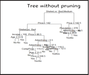
Plot the tree

cv-tree-without-pruning


plot(tree_model)
# add text to the plot
text(tree_model, pretty=0)

Use the model to predict test data target


test_pred = predict(tree_model, testing_data, type="class")

Measure the accuracy of model

Compare the predicted values for target variable 'High' and actual values for it in the testing data set to determine the accuracy of the model

accuracy = mean(test_pred==testing_High)
accuracy
#[1] 0.715
# accuracy is quite low

Use Cross validation to improve accuracy of the tree model

The cross-validation function gives the size and corresponding deviance or error. 'Pruning' the tree model using the size with lowest deviance can help improve the accuracy


# To improve the accuracy we do cross validaion
# cross validation to check where to stop pruning

set.seed(3)

cv_tree = cv.tree(tree_model, FUN = prune.misclass)
names(cv_tree)
# [1] "size" "dev" "k" "method"
# size of prune trees
# dev - deviance or cv error rate

# plot the size and deviance to see where error is lowest

plot(cv_tree$size, cv_tree$dev, type="b",
xlab='Tree Size',
ylab='Error Rate',
main = 'Cross Validation: Error Vs Size')


Interpret the cross-validation plot 

'size' vs 'deviance' cross-validation plot indicates minimum error rate is for size 9. Using this size to prune could help improve accuracy.
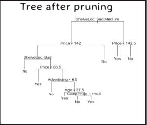
 

cv-error-vs-size


Prune tree model 

Use best size from cross-validation plot for pruning to improve accuracy

# prune the model and plot

pruned_model = prune.misclass(tree_model, best = 9)
plot(pruned_model)
text(pruned_model, pretty = 0)


Compare tree plots before and after pruning

cv-tree-without-pruning

cv-tree-after-pruning

Measure accuracy of pruned model

And compare with the accuracy of tree model before pruning
#[1] 0.715

# test the accuracy of pruned model

tree_pred = predict(pruned_model, testing_data, type="class")

accuracy = mean(tree_pred == testing_High)
accuracy
# [1] 0.77
# Bit improvement compared to 0.71