Machine Learning (ML)
.
Getting Started
I urge you to watch the accompanying video to understand machine learning w.r.t data analysis. Below I have explained my understanding of the topic as simply as I could; and I hope, it helps you to get started on and delve further into ML.
Introduction to Data Analysis using Machine Learning
A must-watch ML presentation By David Taylor

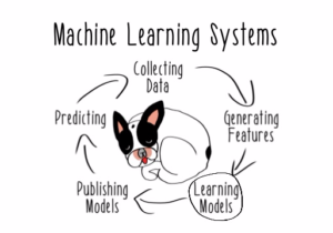
What is Machine Learning?
It is an offshoot of the field of Artificial Intelligence.
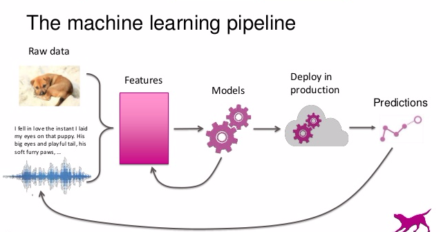
ML is use of algorithms to create knowledge from data. Algorithms are mathematical formulas with if-then loops; and execute like a black box which learns about the data patterns or trends from known data in order to predict an unknown property for new data.
So ML is yielding algorithm to make predictions from data.
.
.
.
.
.
.
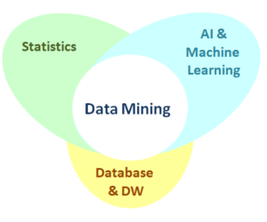
ML is between Statistics and Data mining
Statistics develops methods or models that explain the data, data mining is a task to solve a real world problem where you do not have to care about which method you use. ML develops algorithms or models to solve a specific data analysis task.
.
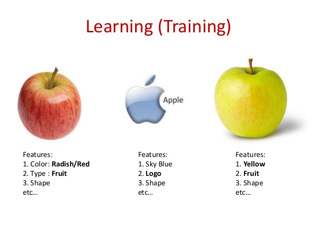
Most fundamental part of ML is Data
Database records in ML are called instances
Database columns in ML are called features
Data instances are represented as feature vectors
Say, for example, you have weight and height for each person, then
Bob --> (175,72) - is a data instance
If you add many other features like blood pressure recorded per day then an instance would look like this
Bob --> (175,72,120,95,130,110.........) - a complex data instance
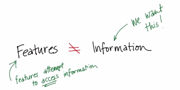
The feature vector should be relevant to the ML task at hand. So if the task is to predict the risk of heart attack the feature vector comprising weight, height, daily blood pressure is useful but for some other task like face recognition it is redundant. Feature engineering is needed to build useful feature vectors for solving specific prediction task.
.
ML is about generalization
ML is about making sense of existing data. Say you have Terabytes of data; using ML you can place similar data points in clusters or groups based on some commonality in features and give a compressed representation like data consists of, say 26 coherent groups and a new data instance is predicted to belong to group #5.
.
ML consists of only three basic methods
Classification
You are given data and you know which group your data instances belong to.
Clustering
We need to figure out which data points sit close to each other
Regression
Data points are ranked based on fitted line called the regression line.
.
Classification and Regression use fairly similar technology as in both methods a prior knowledge of the data is required; difference is that Classification is used for categorical data and Regression for continuous data.
Clustering is more like starting with a clean slate - no prior knowledge of the data is required.
What are Types of Features in ML?.
Features
Dataset columns are features
Instances
Dataset rows are instances
.
Each instance is independent of another, that is, if a value of feature is changed for one instance it would not affect the other instances or rows.
.
Types of Features
.
Numeric
Quantitative data type
.
Interval
Date or Time, Degree Celsius, etc.
Even though they are numbers they can Not be added or divided like numeric features. For example, you can't say that the total temperature for yesterday and today is 60 degree Celsius - that does not make sense.
.
Ordinal
In ordinal type, data is ordered based on the rank
For example, for feature Qualification, having values under-graduate, graduate, post-graduate; the comparison under-graduate < graduate < post-graduate is logical.
.
Categorical
A property or feature for which number can be place holder and the only mathematical function that can be used is "equal to" or "not equal to"
For example, for property Color the values are: red = 1, blue = 2, orange=3 but the comparison red < blue < orange is Not logical.
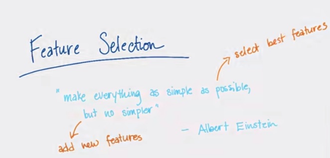
What is the challenge in Machine Learning?
The main challenge lies in features. If you come up with the right features for the ML task the learning model does not have to be sophisticated.
.
What is Normalization?
It is a technique for feature scaling.
Suppose we select two dimensions of a dataset for clustering. One feature has values in thousands and the other in single digits, so in order to make them comparable we can scale them. The two axis for the two dimensions should be in same scale, that is, x-axis and y-axis intervals should be same.
To achieve this, from each unit subtract its mean and divide by its standard deviation (sd) so units are sd away from their respective means.
The same logic can be applied to mutli-dimensional data.
.
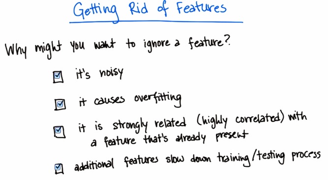
Thorough domain knowledge is important for feature selection and construction. You can leave out features that are not important for the ML task in hand and sometimes you may have to construct new features that have more impact on the prediction.
So focusing on features is essential for solving any ML problem.
What are the types of Machine Learning?
.
There are two kinds of ML:
.
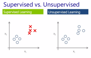
Unsupervised Learning
This is exploratory ML where you do not know what you are looking for. Previous knowledge of data is not required. It explores the raw data for you and gives information of any existing patterns or trends.
.
Supervised Learning
This is predictive ML where the main goal is to use the existing knowledge of the dataset to predict an unknown property for new dataset. It is like statistics where you have a hypothesis and you are trying to prove it - you use properties of a subset of data and apply it to more real world data.
.
.
.
What is a label?
Label is the feature you want to learn from the known data set and predict for the unknown data set.
.
For example: Suppose you have 500 fruits of types apples, oranges and bananas. For each fruit you have the weight, sweetness & acidity measures recorded. Now, say that, while in transit 200 fruits fall off of the truck.
So if you want to predict the type of fruit for the missing 200 using ML, then 'fruit type' is the label; and weight, sweetness & acidity are the features. And based on the knowledge of features of 500 fruits and label information of 300 fruits we can predict the label for the missing 200 fruits.
.
Columns = label + features and are like class definition
Rows = instances of your label & features and are like objects
.
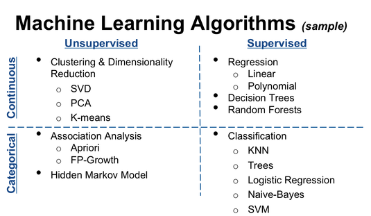
The above "fruit type" prediction is an example of Supervised learning - we start with labels, we have a property we know for some data and we predict that property or label for new data. When label is categorical we use classification, and when label is numerical we use regression, supervised learning algorithms.
.
Unsupervised learning is exploratory analysis and there is no 'label' associated with it. Clustering is unsupervised learning method where the clusters are formed using the features. In our fruit example, if we just scatter plot sweetness vs acidity, we will be able to see high density regions, called clusters, separated by low density regions. These clusters group similar objects but we do not know what they correspond to in the real world.
Say, the three cluster are c1 c2 c3
- c1 is cluster with high acidity and low sweetness
- c2 is cluster with medium acidity and medium sweetness
- c3 is cluster with low acidity and high sweetness
So fruit type with high acidity and low sweetness will be in c1, medium acidity and medium sweetness in c2; and low acidity and high sweetness in c3.
What is Machine Learning Algorithm?
Classification, Clustering and Regression are the three basic methods for ML - the implementation logic for these methods is called algorithm or model.
.
.
.
.
Below are a few data analysis examples, I have implement in R, using ML algorithms:
.
.
.
kNN >> (Work in progress)
.
.
Approaching a Data Analysis problem using ML Algorithms
Define the task you want to achieve using ML
Problem definition is the most important step to measure the success of your ML process. You should spend as much time as possible to first understand the problem you are trying to solve using ML because that is what distinguishes ML from any statistical analysis where the focus is primarily to infer something or prove a hypothesis; whereas, in ML it is imperative to select the right model to solve the single task of prediction as defined by the problem statement.
Understand your data
Feature selection and construction helps in narrowing down a complex data structure. Use unsupervised learning methods like clustering to understand the coherence of the data points. Remove redundant information, combine the features to get more meaningful and relevant data. Once the features that are important for solving the problem are identified, scale them - this is a very important step and should never be skipped. Normalization for scaling is one of the most popular methods. See example...
Evaluate Algorithm
It is easy to select an algorithm once the problem definition is understood. To optimize the results you can adopt the following process:
Optimizing the model:
Test the model with different features, different datasets for training & testing and compare the accuracy. If the accuracy does not change much then the model is optimized to it's best possibility. If the results vary a lot for the different datasets then you may need to reanalyse the feature selection and/or use another model. Sometimes it is good to use an ensemble model which internally uses many simple models on different training sets and uses voting method to select highest accuracy model. See example...
Improving accuracy:
Once a model is selected, accuracy can be improved by tweaking the input parameters to the model. For example, 'pruning' technique can be used to determine the size of tree with minimum error rate for classification tree model or using Silhouette Coefficients to determine the best K in KMeans. See example...
Present the solution
Once you are satisfied with the outcome of your ML, you need to present the solution for the problem definition. Describe the solution such that it will be understood by third parties who are not interested in the nitty gritties of the ML methods but rather in the results.
What is Clustering ?
For solving any data analysis problem it is important to understand the data first. One way to do this is to group similar data points using Clustering algorithm.
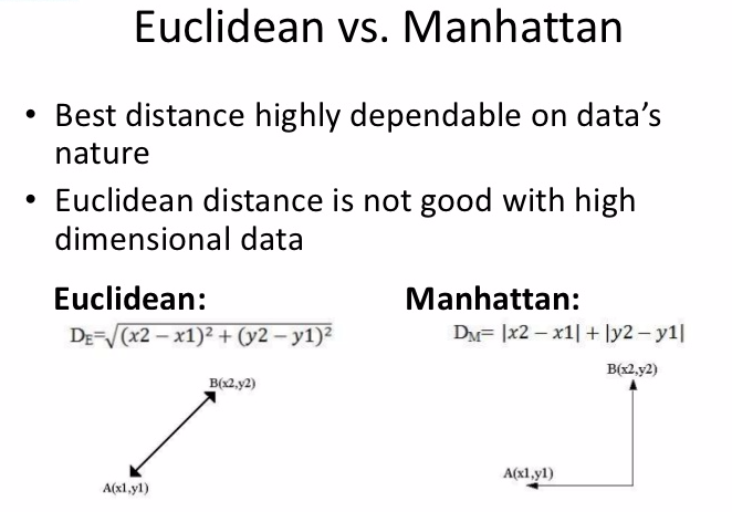
Clustering associates data points by measuring the distance between them. There are two ways to measure that distance:
Euclidean distance - straight line distance between data points. It is the diagonal distance between two data points and most commonly used.
Manhattan distance - orthogonal distance; that is traversing along the sides of right angle instead of the diagonal. Not so common.
.
.
KMeans Clustering
It is the most popular clustering algorithm; use it to get an idea about the data clusters.
.
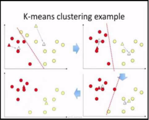
How Kmeans Clustering works?
In Kmeans, k is number of clusters, you need to choose k first. Scatter plot important features to get an idea of number of clusters. For each of the k clusters, a center point is selected called centroid. Data point are assigned to the closest cluster based on their distance from the centroids of the clusters.
After reassigning data points, a new centroid is calculated for each cluster as the mean distance of all the new data points assigned to it. If the new centroids do not change from the previous then the data points remain in the same cluster otherwise the process of reassigning the data points and recalculating the centroids is repeated.
After several runs; if a particular data point gets assigned to two clusters, say out of 100 runs, 48 times to cluster c1 and 52 times to cluster c2, take majority vote and assign it to c2. See example...
.
How to find best k?
It is also a good idea to test with different values of k. One good criterion to decide natural number of clusters, k, is silhouette coefficients which for each data point calculates the ratio of average distance from this point to every other point in the cluster to its minimum distance from a point which is not in the same cluster. Plot the silhouette coefficient for different k values, and select the best k value which is the one corresponding to highest coefficient value.
.
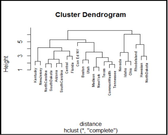
Hierarchical Clustering
We take all the points, connect the points to each other, one by one covering nearby points. So if there are 178 data points and you connect two nearest points then you have one cluster with two points and remaining 176 points. Continue connecting points close to each other thus forming clusters until dense regions are separated by sparse points. The results of hierarchical clustering are usually presented in a dendrogram. See example...
.
.
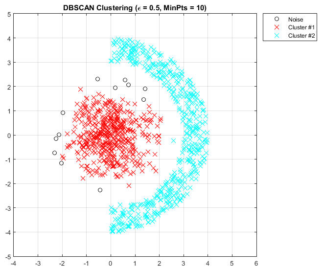
Density-based spatial clustering of applications with noise (DBSCAN)
It is a density-based clustering algorithm; given a set of points in some space, it groups together points that are closely packed together - points with many nearby neighbors, marking as outliers points that lie alone in low- density regions - whose nearest neighbors are too far away. DBSCAN is one of the most common clustering algorithms and also most cited in scientific literature.
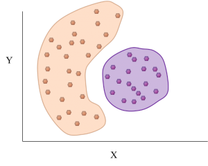
Clusters of different shapes, like globular or looped, are formed by connecting points locally and centrally. You have to give the criteria for density, for example, maximum distance 0.5 from center and minimum 10 points to form high density regions.
.
What is K-NN Algorithm and How is it different from KMeans?
K-nearest neighbors is a classification algorithm, which is a subset of supervised learning. K-means is a clustering algorithm, which is a subset of unsupervised learning.
.
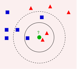
Example of k-NN classification. The test sample (green circle) should be classified either to the first class of blue squares or to the second class of red triangles. If k = 3 (solid line circle) it is assigned to the second class because there are 2 triangles and only 1 square inside the inner circle. If k = 5 (dashed line circle) it is assigned to the first class (3 squares vs. 2 triangles inside the outer circle).
.
In K-NN the number of labels or classes is known, hence it is supervised learning; and the purpose of the algorithm is to classify the unknown data point as one of these classes based on the number of nearest neighbours as set by k.
If k=1 then it is simply the nearest neighbour label that is assigned to it. Suppose two neighbours of different classes are at the same distance then how do we determine which class to assign if k=1? We can use the majority nearest neighbour method to avoid such tie situation.
For n = number of classes:
if n is even then k = n+1
if n is odd then k = n+2
What is Fitting in ML?
Using K-NN example:
If k = 1, then the unknown data point is classified as its nearest neighbor. For k > 1 we use the majority of the nearest neighbors to predict the class. However, if k is very high, the new data points will get assigned the label of the maximum data points; therefore we have to find the optimal value of k for correct classification - this is called fitting an algorithm.
.
Underfitting Vs Overfitting
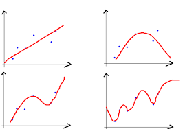
Fitting an algorithm is like fitting a regression line.
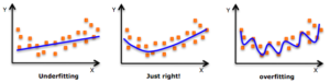
Data points may not always be along the straight line.
Underfitting
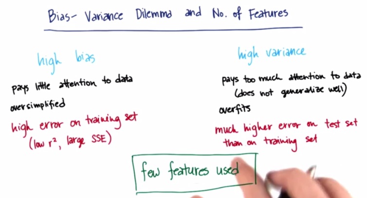
If many points are away from the regression line, it is biased as a line/model is fitted taking into account only few data points thus ignoring the underlying trend formed by most of the data points.
Overfitting
When the model is fitted such that it takes into account deviation in each data point then it is said to be overfitted because it includes noise. Such a model is tightly fitted to the data set and may not predict well for a random data point from the data. For example, if it is tested with an outlier data point it will result in high variance error.
.
Bias-Variance Trade-off Using Training & Test Data
Underfitting - is high bias, low variance
Overfitting - is low bias, high variance
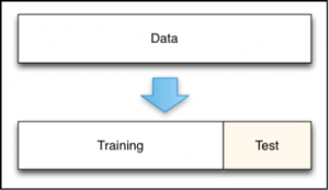
Training & Test Data Set
Balance bias & variance by randomly sequestering part of your
data as a training set and the remaining as test dataset. Training data, say 70 percent of the dataset, is used to create your ML model and Test data, the remaining 30 percent of the dataset, is used to test the accuracy of the model predictions.
Training Phase
Input: Data instances and their true labels
Output: Classifier or classification model
Test Phase
Input: A data instances
Output: Its label
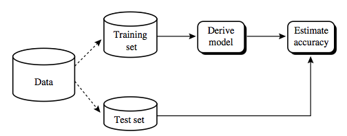
Measuring Accuracy
Use the confusion matrix, pivot table, to compare the actual values and the predicted values for the Test data set using the Training model. If the accuracy is in the desirable range and does not change for the different random samples of Training and Test data we can assume that the model is fitted just right. If otherwise, that is accuracy differs a lot from sample to sample, then you might have to look at other parameter optimization of the model or another model or ensemble model.
For example, in K-NN, for different k values, train/test the model with randomly selected data and compare the predictions. If for a given k value the accuracy does not change it be the best fit model. You can also plot the learning curve using Error Vs k.
What is Cross Validation?
Underfitting a model can lead to high bias by omitting important data points that influence the data trend and overfitting a model can lead to high variance by including all the data points resulting in noise overlooking the actual trend of the data. To trade-off between these errors caused by bias & vairance we divide he dataset into two parts, one part to train the model and the other to validate or test the model against. The data points are shuffled and divided based on a certain ratio, say 70:30 or 50:50, to form the training and test datasets.
.
.
Cross validation provides techniques to iteratively partition the dataset into multiple training & test datasets, for the given model and calculate its accuracy by averaging out the test predictions.
.
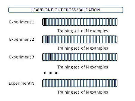
Leave One Out Cross Validation technique (LOOCV)
If there are n data points, and we take n-1 data points to train the model and test against the remaining single data point. The process is iterated for each data point. This approach is tedious and prone to high bias as training data set has most of the data points. Also, it can lead to high variance if the left out data point is an outlier.
To overcome these problems the LOOCV strategy is extended to collective data points forming groups or folds - called k-fold cross validation and applying LOOCV to the folds instead of the data points.
.
.
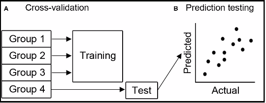
K-Fold Cross Validation
In k-fold cross-validation, the original sample is randomly partitioned into k equal sized subsamples. Of the k subsamples, a single subsample is retained as the validation data for testing the model, and the remaining k − 1 subsamples are used as training data. The cross-validation process is then repeated k times (the folds), with each of the k subsamples used exactly once as the validation data. The k results from the folds can then be averaged to produce a single estimation. The advantage of this method is that all observations are used for both training and validation, and each observation is used for validation exactly once. 10-fold cross-validation is commonly used but in general k remains an unfixed parameter.
When k = n (the number of observations), the k-fold cross-validation is exactly the leave-one-out cross-validation. k-fold Cross Validation - Wikipedia
.
See example Cross Validation of Tree model
What is Skewed Data?
A skewed data distribution is one which is not symmetrical about the mean, or average.
Mean is calculated using value of all the data points and hence it is a representation of entire dataset. However, when data points stray far away from each other then this value is no longer a good representation of the data distribution. Mean and Mode(most frequently occurring value) are not close to the Median(the middle value).
.
No Skew
Normal Distribution.
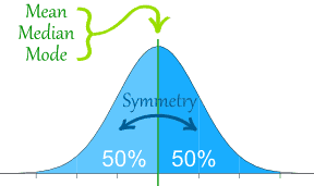
When the data points are around the central point, median, and there are no extreme values deviating from median value then three is no skew. The mean and mode are near median and such balanced data distribution forms a bell curve.
.
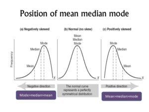
Positive Skew
Right Long Tail
When the data points deviate from the central point, median, more towards the right then there data is positively skewed. The extreme values are on the right side hence the mean is greater than the median and such a data distribution forms a long tail on the right side of the bell curve.
.
Negative Skew
Left Long Tail
Similarly, when there are extreme values to the left of median there is negative skew and mean is less than the median. Such a data distribution forms a long tail on the left side of the bell curve.
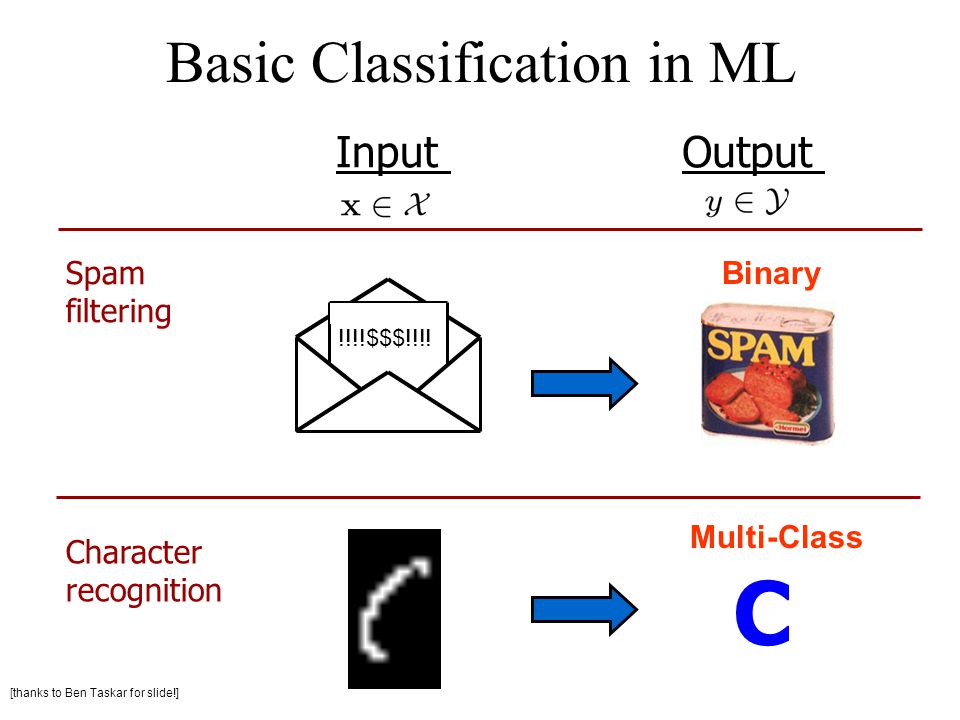
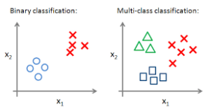
What is Multi-Class Classification?
When there are only two classes for the give dataset it is called binary class data.
In machine learning, multiclass or multinomial classification is the problem of classifying instances into one of the more than two classes (classifying instances into one of the two classes is called binary classification).
While some classification algorithms naturally permit the use of more than two classes, others are by nature binary algorithms; these can, however, be turned into multinomial classifiers by a variety of strategies.
Multiclass classification should not be confused with multi-label classification, where multiple labels are to be predicted for each instance.
.
What is Curse of Dimensionality?
When there are many many features (few dozen to many thousands) in the dataset it is called high dimensional data.
Such high-dimensional spaces of data are often encountered in areas such as medicine, where DNA microarray technology can produce a large number of measurements at once, and the clustering of text documents, where, if a word-frequency vector is used, the number of dimensions equals the size of the vocabulary.
Multiple dimensions are hard to think in, impossible to visualize; and, due to the exponential growth of the number of possible values with each dimension, complete enumeration of all subspaces becomes intractable with increasing dimensionality. This problem is known as the curse of dimensionality.
.
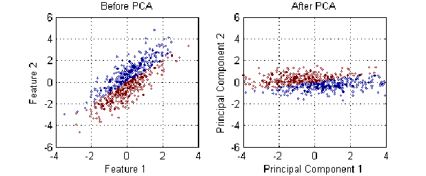
Dimensionality Reduction Using PCA
Dimensionality reduction can help solve the problem of high dimentionality. Principal component analysis (PCA) is a statistical procedure that uses an orthogonal transformation to convert a set of observations of possibly correlated variables into a set of values of linearly uncorrelated variables called principal components.
PCA removes the correlated variables and identifies the most influential uncorrelated variables called 'principal components' in terms of causing maximum variance. Thus, PCA reduces number of predictors (features used in prediction model) by reducing multi-collinearity.
.
Principle Component Analysis (PCA) clearly explained
By Joshua Starmer
What are the different Classifiers?
.
K-NN (K-Nearest Neighbors)
In K-NN method the classifier requires measuring the distance of each data point from every other data point in the data set. This can be tedious for big volume of data even if we use subsets of the dataset for Training and Test phases; it does not scale that well when there are millions of data points and ML is all about scaling.
SVM (Support Vector Machine)
SVM can help overcome the problem of measuring the distance between data points by using a hyperplane that divides the data space and makes it easy to classify the data points based on which side of the hyperplane they are in.
In geometry a hyperplane is a subspace of one dimension less than its ambient space. If a space is 3-dimensional then its hyperplanes are the 2-dimensional planes, while if the space is 2-dimensional, its hyperplanes are the 1-dimensional lines.
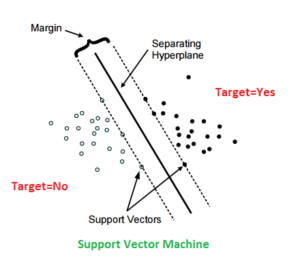
We build a line or hyperplane that would separate data points. In the above figure a good line is one that is maximum distance from solid dots and empty dots - it is called maximum margin classifier and the dots that define the slope of the line are called support vectors. To classify a test data instance all you have to see is on which side of the plane or line the dot lies - there is no need to calculate the distance from any other data instance.
SVM Challenge
The challenge in SVM is the mathematical complexity of calculating the hyperplane.
SVM for non-linear data
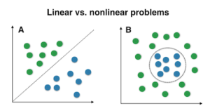
Data points may not always be linearly separable and SVMs are really good at solving non-linear classification problem. The complexity of the algorithm does not increase for non-linear classification
SVM for Skewed Class
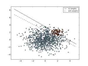
SVM is awesome for skewed data with binary classes - that is there are two classes and the data points are skewed to either one of the calss types. Once the SVM line is drawn all that matters is the support vectors and other points can be ignored.
SVM Limitations For Multi-Class
SVMs For High Dimensional data
Below are two instances of typical real world high dimensional data, they're usually very long and sparse.
Data instance 1 : (0,0,0,0,0,0,0,0,2,0,0,0,0,0,2,0,0,0,0,0,0,0,0,0,0,0,0,
2,0,0,0,0,0,2,0,0,0,0,0,0,0,0,0,0,0,0,2,0,0,0,0,0,2,0,0,
0,0,0,0,0,0,0,0,0,0,2,0,0,0,0,0,2,0,0,0,0)
Data instance 2:(0,0,0,0,0,0,0,0,1,0,0,0,0,0,1,0,0,0,0,0,0,0,0,0,0,0,0,
1,0,0,0,0,0,2,0,0,0,0,0,0,0,0,0,0,0,0,2,0,0,0,0,0,1,0,0,
0,0,0,0,0,0,0,0,0,0,1,0,0,0,0,0,10,0,0,0,)
The above instances are similar in the sense that most of the features are zero.
So, in high dimensional data, geometry is non-intuitive but classes can be linearly separable.
When do we use SVM?.
When there is Not much training data available with the labels
- Training SVMs is computationally expensive
- A million instances would be upper limit.
When the data has geometric interpretation for the ML task at hand
- For example, in Computer Vision problems that processes pictures.
When high precision is crucial
- SVM will not give the desired accuracy right away but with continuous work and parameter tuning accuracy up to 90 percent can be achieved
.
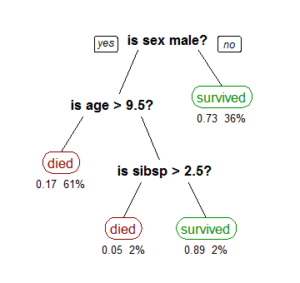
Decision Trees
SVMs are not good for multi-class data and this is overcome by Decision Trees classifiers that are best for high multi-class & high dimensional data.
A tree showing survival of passengers on the Titanic ("sibsp" is the number of spouses or siblings aboard). The figures under the leaves show the probability of outcome and the percentage of observations in the leaf.
Decision Trees Challenge
Decision Trees are like a game of twenty questions; where based on the answer you eliminate 50 percent of possibilities. For example, trying to identify a famous personality you ask the below questions to arrive at the answer:
First Strategy:
- is this person male or female
- is this person politician or not
- and so on
Second Strategy:
- is it Indira Gandhi - No
- is it that guy - No
- is it my neighbor (whom you have never met)
As you can see clearly, in strategy one, you could get closer to the answer a lot quicker than with second one, which could take 7.5 billion guesses, if going thru every person in the world.
So the main challenge in Decision Trees is setting up the questions. Information gathering at every question; that is, information gain at each step of separation is the idea behind Decision trees. Understanding of features is important for setting up Decision Tree splitting questions.
.
Classifier Ensemble (Decision Forest)
Decision Trees are simple but as stand alone they are not that good as compared to using ensemble of Decision Trees called Decision Forest.
Decision Tree analyses the data, places twenty questions such that it can split data to give maximum information or a 50-50 split. If you run the decision tree with different training data and the result look very different for different training sets then this is indication that your not fitting correctly . Use ensemble methods in such case.
Decision Forest uses high biased model, that underfits your data, run simultaneously with different parameters and averages out the result thereby adding complexity to your model and fits better. It can also use a high variance model, which tries to fit each point, that fits noise, run that several times and average out such you get a less complex model.
Random Forest is a ensemble model that takes a bunch of decision trees without caring for the maximum information gain split and uses voting for best fit. With Random Forest you can use few most important features to improve accuracy; for sake of comparison, run the model with two least important features and compare the accuracy using confusion matrix, it should fall. See example...
.
Boosted Decision Trees
Build a decision forest iteratively. Choose new trees for cases not yet covered by the current version of the forest, or for which portions of training data have not been covered well.
Once you build millions of trees like that, it is the best method in universe for prediction. This very powerful technique is used in the current state-of-the-art web search.
When do we use boosted trees?
- On high multi-dimensional data. For example, text classification
- In high multi-class classification setups. We can have as many classes as the number of leaves in the trees
- When classes are Not too skewed in size. If we have 10 positive instances and 1 million negative ones, chances are high that all trees will always say "no"
.
Logistic Regression
Another very popular classifier that, confusingly, does classification as well as regression. It estimates the probability of an event occurring.
The formula is ratio of probability of positive event occurring by the probability of negative event occurring which is proportional to the linear combination of features. You add log to the ratio so that the probabilities are between 0 and 1.
For example, to find if person would be good at basket based on given height and weight, the logistics regression formula would be
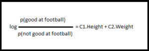
p is the probability and C2 & C2 are the coefficients for the features Height and Weight respectively.
Logit Regression Challenge
The challenging part is learning the coefficients. The coefficients is positive for positive features and negative for negative feature. So in this case C1 will be positive and C2 will be negative because for basketball player a good height is more desirable than a heavy body.
When do we use Logistic Regression?
- In probabilistic setups. Easy to incorporate prior knowledge
- When the number of features is pretty small. The model will tell you which features are important. Good "explainability" about the features
- When you want to train the model really fast. Training Logistic Regression models is relatively fast
- When precision is not that crucial. Logistic Regression is really not the best algorithm for precision
What is Cost Function?
Cost Function is cost of mis-classifications. In accuracy we treat each mis-classifcation as equal. For example, if apple is classified as pear it is no worse or better than apple being classified as orange. In certain cases we can optimize these penalties for wrong guesses, so that we can penalize events that we do not want at all.
Common cost function use is to penalize false negatives more than false positive or vice-versa.
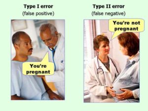
For example consider the below diagnosis :
"You are pregnant" - is a positive statement
"You are not pregnant" - is a negative statement
Now, if a man is given diagnosis:
"You are pregnant" - it is False Positive and
"You are not pregnant" - it is True Negative
And, if a woman with big belly is given diagnosis:
"You are pregnant" - it is True Positive and
"You are not pregnant" - it is False Negative
.
False Positive Vs. False Negative
In what kind of classifier would it be more important to minimize false positives or false negatives?
Example 1: An adult-content filter for school computers
"Content is Adult" - Positive statement
"Content is Not Adult" - Negative statement
Kids' movie is classified as "Content is Adult" - False Positive
Porn is classified as "Content is Not Adult" - False Negative
In this case False Negative error should be minimized; in the context of school it is okay to mis-classify a Kids' movie as porn but it is definitely not acceptable to pass a porn as a suitable content for school computers.
Example 2: A genetic risk classifier for cancer
"You have cancer" - Positive statement
"You do not have cancer" - Negative statement
If a cancer-free patient is diagnosed as "You have cancer" - it is a False Positive
If a cancer patient is diagnosed as "You do not have cancer" - it is a False Negative
In this case also False Negative error will cost more; it is far worse to not detect cancer in a patient who has cancer than to detect cancer in a patient who doesn't have.
Summary.
The attached video, according to me, is one of the best presentations on ML basics for beginners and based on my understanding of it I have listed a few of the best practices in ML below.
Machine Learning: The Basics, with Ron Bekkerman
See Handwriting Recognition using
Decision Tree example @31:57
What are the best practices in ML?
.
Tip 1 : Adopt domain-specific approach
Don't just use a generic solution to the data analysis problem. Understand your data and the specific problem you are trying to solve. You can achieve up to 80 percent accuracy without ML; if you want to improve the performance use ML
.
Tip 2 : Scrutinize the features
Most of the signals are in features. Feature engineering is very important step in solving the data analysis task using ML.
.
Tip 3 : Improve the crowdsourced labels
This can improve precision from 80 percent to 95 percent.
.
Tip 4 : First cluster features
For very sparse, highly multi-dimensional data first cluster features and represent data instances as dense vectors of feature clusters; then apply classifier on these representations
.
Tip 5 : Choose the right classifier for your task
Most of the classifiers are open sourced.
.
Tip 6 : Ensemble
Mix all classifiers into one big ensemble; this is one of the most effective ways to improve accuracy.
.
Case Study
Work-in-progress