RL Characteristics
![]()
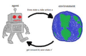
- There is no supervisor, only a reward signal – it is a trial and error approach, there is no one to say to do that in a given situation. There are points/rewards but no one can say that is the best action
- Feedback is delayed - you can see the result of the decision taken after many many steps, it’s only retrospectively that you realize whether the decision was good or bad.
- Time really matters – it is not classical Supervised Learning setting where you get dataset on which you train and test your model, the data at each step is correlated to its earlier step. Example, imagine a robot, depending on where it moves it sees new data and decides where to move ahead.
- Agent’s actions affect subsequent data it receives – it’s like an active learning environment with the objective of optimizing the result.
RL Examples
![]()
- Fly stunt manoeuvres in a helicopter – you control the helicopter and make manoeuvres. There is a positive reward for following the desired trajectory or when the helicopter comes within a radius of where we want it to be and a large negative reward for crashing so that it learns that it is bad to crash.
- Build a machine to defeat the world champion at the game of chess – positive/negative reward for winning/losing a game; at the end of the game, it knows if it has won or lost. The agent will figure out for itself how to optimize the rewards and make decisions along the way to maximize the rewards at the end of the game.
- Manage investment portfolio where investment agent is getting data at real-time and decides where to invest – in which financial product such that the reward (money) is maximum. There is a positive reward for each Rupee in the bank.
- Make a humanoid robot walk – a positive reward for forwarding motion and a negative reward for falling over. To make it walk across the room, you check if it is making progress at each step and you don’t want it to fall over. At each step, there is a reward and it needs to figure out to walk across the room based on that.
- Play Atari games better than humans.
RL Framework
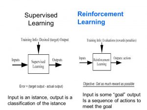
Supervised Learning - Input is an instance, the output is a. classification of the instance.
Reinforcement Learning - Input is some 'goal', the output is a sequence of actions. meet the goal.
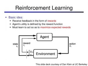
Reinforcement learning is based on the reward hypothesis:
All goals can be described by the maximization of the expected cumulative reward.
A reward Rt is a scalar feedback signal which indicates how well the agent is doing at step t and the agent’s job is to maximize the cumulative reward.
We use the below RL framework to solve the RL problems. RL problem is one of sequential decision making with the goal to select actions to maximize total future reward. So we have to think ahead because actions may have long term consequences, rewards may be delayed and sometimes you may have to sacrifice immediate rewards to gain more long term rewards.
For example, a financial investment may take months to mature so you are losing money now but in the end you may get more money; for refuelling a helicopter you have to stop your manoeuvring thereby lose rewards but it might prevent a crash in several hours; in a chess game you make a move to block the opponent which might help to improve winning chances many many moves from now…
Agent and Environment Interface
History and State:
Ht = A1,O2,R2,A2,O3,R3…At-1,Ot,Rt
St = f(Ht)
Agent State:
Sta = f(Ht)
Information State aka Markov State:
A state St is Markov if and only if
P[ St+1|St ] = P[ St+1|S1,..,St ]
St+1 – is the future state
St – is the current state
S1,..,St – is the history of all states until current time-stamp t
![]()
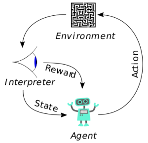
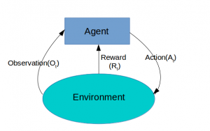
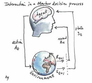
Agent
The agent is the algorithm which decides what actions to take, for example, what financial investment product to buy or what moves to make in the case of a humanoid robot. Those actions are taken based on what observations are made, that is the inputs/reward received by the agent for the actions. It’s a loop where the agent interacts with the environment and influences the environment by the actions it takes. This interaction goes on and on generating a time series of actions and rewards.
At each step t:
- the agent executes action At and receives observation Ot+1 and scalar reward Rt+1
- the environment receives action At and emits observation Ot+1 and scalar reward Rt
- t increments at environment step
History and State
History is the sequence of observations, actions, rewards – that is, all observable variables up the time t.
Ht = A1,O2,R2,A2,O3,R3…At-1,Ot,Rt
The agent or the algorithm builds a mapping from this history to pick an action. The environment looks at what happens due to action and it also looks at history to decide what observation it is going to emit in the next time stamp. So what happens next depends on the history – the agent selects the actions and the environment selects the observations/rewards.
State captures the history in a useful form – it is a function of history
St = f(Ht)
It is summary information that is used to determine what happens next. Depending on the RL problem the state can capture information of last observation or last few observations and as such it can replace entire history and present all the information in a more useful format.
There are many definitions of state, let’s look at the below three:
Environment State – it is the environment’s private representation of observable variables, i.e. it is basically the information used within the environment to determine what happens next - to pick the next observation/reward. The environment state is usually not visible to the agent and even if it is visible it may contain irrelevant information. For example, imagine a robot interact with the real world - that real environment is a set of numbers that determines where the robot is going to move, it doesn’t need to know about all the atomic configuration and other thing but rather only a set of numbers that is going to determine what is going to happen next from the environment perspective – what observation/reward to emit.
Agent State – the environment state doesn’t tell us anything useful for building our algorithm which only sees the observations and rewards coming out of the environment. So we look at the agent state which is a set of numbers that lives within the algorithm. We use these set of numbers to capture what’s happened in the agent so far and summarize that information to help pick the next action. It is our decision what information to capture and what to throw away. It is the information used by reinforcement learning algorithms and it can be any function of history Sta = f(Ht)
Information State aka Markov State – contains all useful information from the history. It is a more mathematical definition of state which basically says that the probability of the next state conditioned on the state you are in is the same as the probability of the next state if you are showed all of the previous states. In other words, you can throw away all of the previous states and just retain the current state, you will get the same characteristics of the future.
A state St is Markov if and only if
P[ St+1|St ] = P[ St+1|S1,..,St ]
St+1 – is the future state
St – is the current state
S1,..,St – is the history of all states until current time-stamp t
Markov Property
The future is independent of the past given the present
H1:t à St à Ht+1:∞
Once the state is known the history may be thrown away.
![]()
The state is sufficient statistic of the future. So, what it says is that if you have the Markov Property then the future is independent of the past given the present. In other words if you have got the state representation St and it is Markov then you can throw away rest of the history as it will not give you any more information of what will happen in the future than the state you have because that state characterizes everything about the future – all future observations, actions and rewards.
St is more compact to work with than entire history.
The distribution of events that might happen to us conditioned on the current state is the same as conditioned on the entire state. So if we make decisions based on St they will still be optimal because we have not thrown away information.
For example, in case of helicopter manoeuvring case, if it is Markov, then its current position & velocity, wind direction can help us determine what will be its next position – we don’t need to know what its position was 10 minutes ago. You don’t need to remember the history of its previous trajectory because it is irrelevant.
Now, in contrast, if you took the imperfect state representation, that is non-Markov – like you have the position of the helicopter but not the velocity, in such case where the helicopter is now will not determine where it will be next because you don’t know how fast it is moving. You will have to look back at history to figure out what its momentum is and that sort of other information.
So we always have to come up with a Markov state to solve the RL problem and our job is to find the State representation that is useful and effective in predicting what happens next.
Markov Decision Process (MDP)
Layering on Markov Property – we add complexity to the basic idea of Markov Property by adding rewards for being in a particular state thus to get Markov Reward Process (MRP) and then by adding actions to move to a particular state thus to get Markov Decision Process (MDP).
![]()
So we start with basic agent – the real brain, the algorithm, which interacts with the environment described in terms of numbers represented as state and then apply some tools to understand it and that is MDP.
A fully observable environment is one in which the agent directly observes the environment, that is
Agent State = Environment State = Information State
Formally this is called Markov Decision Process (MDP) where the agent can see all the numbers in the environment and use that information to come up with the Markov State.
Markov decision processes formally describe an environment for reinforcement learning. Where the environment is fully observable, that is the current state completely characterizes the process. Almost all RL problems can be formalized as MDPs. Partially observable problems can be converted into MDPs.
Bandits are MDPs with one state. It is one of the simplest cases in which there is a set of actions and you are given a reward for an action.
For example, you present an advert to a user on the internet – it either gets clicked or doesn’t and your goal is that it should get clicked maximum times.
Discrete-time stochastic control process
MDP is a discrete-time stochastic control process.
It provides a mathematical framework for modelling decision making in situations where outcomes are partly random and partly under the control of a decision maker.
Markovian Property of MDP: Only the Present Matters
- It is not related to any of the states the agent visited previously
- The solution to the MDP problem is policy (π)
- An Optimal Policy (π*) maximizes long term cumulative reward problem
At each time step, the process is in some state s, and the decision maker may choose any action a that is available in state s. The process responds at the next time step by randomly moving into a new state s', and giving the decision maker a corresponding reward Ra(s,s').
The probability that the process moves into its new state s' is influenced by the chosen action. Specifically, it is given by the state transition function Pa(s,s'). Thus, the next state s' depends on the current state s and the decision maker's action a.
But given s and a, it is conditionally independent of all previous states and actions; in other words, the state transitions of an MDP satisfies the Markov property.
MDPs are useful for studying optimization problems solved via dynamic programming and reinforcement learning.
Markov Process Chains
How Markov Process Chains are formed?
The core problem of MDPs is to find a "policy" for the decision maker: a function π that specifies the action π(s) that the decision maker will choose when in state s.
Once a Markov decision process is combined with a policy in this way, this fixes the action for each state and the resulting combination behaves like a Markov chain :
Since the action chosen in state s is completely determined by pi(s) and Pr(st+1=s'|st=s,at=a) reduces to Pr(st+1=s'|st=s), a Markov transition matrix.
The goal is to choose a policy π that will maximize some cumulative function of the random rewards, typically the expected discounted sum over a potentially infinite horizon:
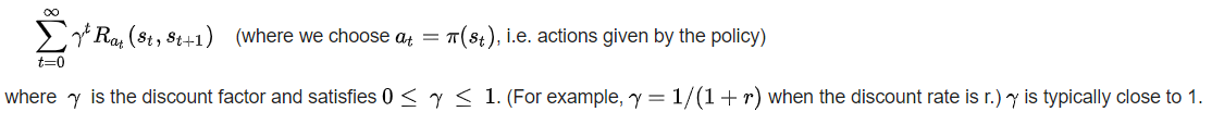
Because of the Markov property, the optimal policy for this particular problem can indeed be written as a function of s only, as assumed above.
The discount factor is used so that the decision maker favours taking actions early and doesn't postpone them indefinitely.
Markov Reward Process (MRP)
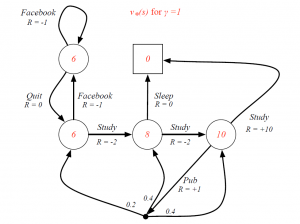
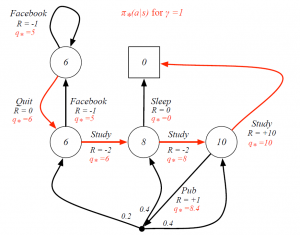
Optimal Value Function for Student MDP
Optimal Action-Value Function for Student MDP

Optimal Policy For Student MDP
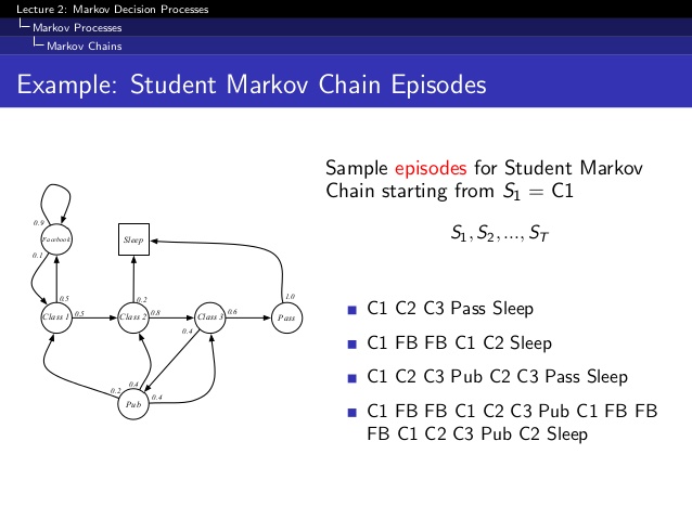
Markov Process or Markov Chain
A Markov Process is a memory-less random process, that is, a sequence of random states S1,S2,… with the Markov Property. It is represented as a tuple < S, P > where S is a finite set of states and P is the transition probability matrix.
Pss’ = P[ St+1=s’|St=s]
Markov Reward Process
A Markov Reward Process is a Markov chain with values. It is represented as a tuple < S, P, R, γ >, where R is the reward function and γ is a discount factor
Rs = E[ Rt+1 | St=s ]
γ ϵ [ 0,1 ]
So, MRP is an MP with some value judgment to decide how good it is to be in some particular state. R tells us how much reward do we get from that state at that moment and discount factor is used to calculate the accumulated reward for the sample sequence of states with rewards discounted over the sequence.
Reward is the immediate value we get for being in a particular state and our objective is to maximize the accumulated reward.
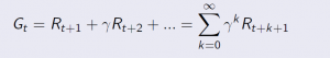
Return
The return Gt is the total discounted reward from time-stamp t
![]()
![]()
Our goal is to maximize the Gt that is the sum of rewards overall time-stamps into the future. But we’re going to discount the rewards by the discount factor γ for each time-stamp infinitely into the future.
γ is the present value of future rewards.
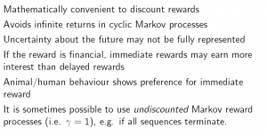
Why discount rewards?
Most Markov reward and decision processes are discounted. Why?
![]()
γ – the discount factor is how much the agent care about the reward it’s going to get in the future. Value close to 0 indicates immediate rewards are more important than future rewards and vice versa if its value is closer to 1.
So, if I’m at time-stamp 10 and I know I’m going to get the reward at step 20 then I should discount that an additional 10 times. The value of receiving reward ‘R’ after k+1 time-stamps is γkR
Discount factor is less than 1 so that the infinite sum can be made finite – for mathematical convenience of converging certain algorithms. Also, in the real world, a decision maker cannot always be certain about the environment – the next action could just lead to the end, no reward at all. For example, in the case of manoeuvring helicopter, it could just crash or in case of robot, the discount factor accommodates the probability that the robot gets switched off.
Also, the discount factor takes care of general animal/human behaviour for instant gratification – immediate rewards are usually preferred due to the uncertainty of future rewards. However, in cases where the sequences are sure to get terminated then the rewards can be undiscounted as there is certainty of the end state.
Value function V(s)
The value function v(s) gives the long-term value of state s
For an MRP v(s) is the expected return starting from state s
v(s) = E [ Gt | St = s ]
Gt = Rt+1 + γRt+2 + γ2Rt+3+…
It shows how good it is to be in a particular state, how much reward can we expect to get if we take a particular action to estimate how well are we doing in a particular state. It is the prediction of the future reward used to evaluate the goodness/badness of states to select between actions that give the maximum reward.
![]()
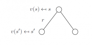
Bellman Equation for MRPs
The value function can be decomposed into two parts:
- immediate reward Rt+1
- discounted value of successor state γ*v(St+1)
v(s) = E [ Gt | St = s ]
# expanding Gt
v(s) = E[ Rt+1 + γRt+2 + γ2Rt+3+… | St=s ]
v(s) = E[ Rt+1 + γ(Rt+2 + γRt+3 + γ2Rt+4 + …) | St=s ]
v(s) = E[ Rt+1 + γGt+1 | St=s ]
v(s) = E[ Rt+1 + γv(St+1) | St=s ]
Rt+1 – is immediate reward for being in state s, i.e. Rs
v(St+1) – value for being in new state s’, which is the probability of transitioning to that sate multiplied by the rewards for being in that state
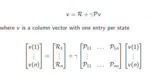
Therefore,
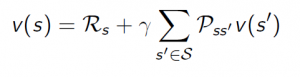
The above Bellman equation can be expressed concisely using matrices
Model-based Vs Model-free Agents
Model
It is the agent’s representation of the environment, what the agent thinks how the environment works.
A model predicts what the environment will do next.
Transitions P – predicts the next state
Pss’ = P[ S’=s’|S=s, A=a ]
Reward R – predicts the next immediate reward
Rs = E[ R| S=s, A=a ]
These three pieces, policy, value function and model – all may or may not be used.
Value-based RL agents use only value function, no policy (implicit).
Policy-based use a policy and no value function.
Model-Free use policy and/or value function but no model. We don’t try to understand the environment – how the environment works. Using Q-learning.
Model-based use policy and/or value function.
See Model-free GridWorld Example and Model-free GridWorld Example.
What is Dynamic Programming?
It is a method of solving problems by breaking them down into sub-problems. So by solving the sub-problems, you can combine the solutions to address the complete problem.
Dynamic Programming is a very general solution method for problems which have two properties:
Optimal sub-structure – Principle of optimality applies, the optimal solution can be decomposed into sub-problems.
Overlapping sub-problems – Sub-problems recur many times. Solutions can be cached and reused.
Markov decision processes satisfy both properties – Bellman equation gives recursive decomposition and Value function stores and reuses solutions
Planning by Dynamic Programming
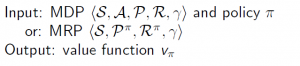
Dynamic programming assumes full knowledge of the MDP. It is used for planning in an MDP.
The prediction method is to evaluate the future given a policy.
The control method is to optimize the future by finding the best policy.
For prediction:
Or for Control:
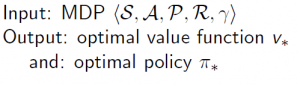
Optimal Policy (π*)
(Source: Reinforcement Learning in R, by Nicolas Pröllochs, Stefan Feuerriegel)
The agent & environment interaction is an iterative process with the goal to maximise the cumulative reward, as shown in the figure below.
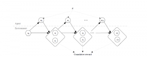
Based on the current state si in step i, the agent picks an action ai ∈ Asi ⊂ A out of the set of available actions for the given state si.
Subsequently, the agent receives feedback related to its decision in the form of a numerical reward ri+1, after which it then moves to the next state si+1.
This knowledge can be used to infer the optimal behaviour, that is the policy/rule that maximises the expected reward from any state.
The optimal policy π* maximizes the overall expected reward or, more specifically, the sum of discounted rewards given by
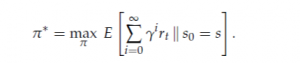
![]()
Q-learning - Model-free Approach
Q(si,ai) - state-action function
The objective of reinforcement learning is to determine a policy π(si, ai) that defines which action ai to take in state si. In other words, the goal of the agent is to learn the optimal policy function for all states and actions.
To do so, the approach maintains a state-action function Q(si, ai), specifying the expected reward for each possible action ai in state si.
In practice, one chooses the actions ai that maximize Q(si, ai). A common approach to computing this policy is via Q-learning. As opposed to a model-based approach, Q-learning has no explicit knowledge of either the reward function or the state transition function. Instead, it iteratively updates its action-value Q(si, ai) based on past experience. Alternatives are, for instance, SARSA or temporal-difference (TD) learning, but these are less common in practice nowadays.
Exploration to Compute Q
Reinforcement learning performs an exploration in which it randomly selects action without reference to Q. Thereby, it collects knowledge about how rewarding actions are in each state.
One such exploration method is ε-greedy, where the agent chooses a random action uniformly with probability ε ∈ (0, 1) and otherwise follows the one with the highest expected long-term reward. Mathematically, this yields
![]()
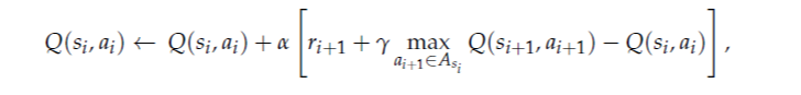
Q-learning algorithm - Update Rule
The Q-learning algorithm starts with arbitrary initialization of Q(si, ai) for all si ∈ S and ai ∈ A. The agent then proceeds with the aforementioned interaction steps:
- it observes the current state si
- it performs an action ai
- it receives a subsequent reward ri+1 after which it observes the next state si+1
Based on this information, it then estimates the optimal future value Q(si+1, ai+1), i.e. the maximum possible reward across all actions available in si+1. Subsequently, it uses this knowledge to update the value of Q(si, ai). This is accomplished via the update rule with a given learning rate α and discount factor γ.
Thus, Q-learning learns an optimal policy while following another policy for action selection. This feature is called off-policy learning.
Batch Reinforcement Learning
(Source: Reinforcement Learning in R, by Nicolas Pröllochs, Stefan Feuerriegel)
Reinforcement learning generally maximizes the sum of expected rewards in an agent-environment loop. However, this setup often needs many interactions until convergence to an optimal policy. As a result, the approach is hardly feasible in complex, real-world scenarios.
A suitable remedy comes in the form of so-called batch reinforcement learning, which drastically reduces the computation time in most settings.
![]()
How Batch Learning saves time?
Different from the previous setup, the agent no longer interacts with the environment by processing single state-action pairs for which it updates the Q-table on an individual basis.
Instead, it directly receives a set of tuples (si, ai, ri+1, si+1) sampled from the environment. After processing this batch, it updates the Q-table, as well as the policy. This procedure commonly results in greater efficiency and stability of the learning process, since the noise attached to individual explorations cancels out as one combines several explorations in a batch.
Batch Reinforcement Learning
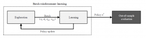
The batch process is grouped into three phases.
- In the first phase, the learner explores the environment by collecting transitions with an arbitrary sampling strategy, e.g. using a purely random policy or ε-greedy. These data points can be, for example, collected from a running system without the need for direct interaction.
- In a second step, the stored training examples then allow the
agent to learn a state-action function, e.g. via Q-learning. The result of the learning step is the best possible policy for every state transition in the input data. - In the final step, the learned policy can be applied to the system. Here the policy remains fixed and is no longer improved.
Experience Relay
(Source: Reinforcement Learning in R, by Nicolas Pröllochs, Stefan Feuerriegel)
Another performance issue that can result in poor performance in reinforcement learning cases is that information might not easily spread through the whole state space.
For example, an update of
Q-value in step i of the state-action pair (si, ai) might update the values of (si-1, a) for all a ∈ Asi .
![]()
However, this update is not back-propagated immediately to all the involved preceding states. Instead, preceding states are only updated the next time they are visited. These local updates can result in serious performance issues since additional interactions are needed to spread already-available information through the whole state space.
As a remedy, the concept of experience replay allows reinforcement learning agents to remember and reuse experiences from the past.
The underlying idea is to speed up convergence by replaying observed state transitions repeatedly to the agent as if they were new observations collected while interacting with a system.
Experience replay thus makes more efficient use of this information by resampling the connection between individual states. As its main advantage, experience replay can speed up convergence by allowing for the back-propagation of information from updated states to preceding states without further interaction.
Conclusion
(Source: Reinforcement Learning in R, by Nicolas Pröllochs, Stefan Feuerriegel)
Reinforcement learning has gained considerable traction as it mines real experiences with the help of trial-and-error learning.
In this sense, it attempts to imitate the fundamental method used by humans to learn optimal behaviour without the need for an explicit model of the environment.
![]()
Reinforcement Learning with R programming
In contrast to many other approaches from the domain of machine learning, reinforcement learning solves sequential decision-making problems of arbitrary length and can be used to learn optimal strategies in many applications such as robotics and game playing.
Implementing reinforcement learning is programmatically challenging since it relies on continuous interactions between an agent and its environment. To remedy this, the ReinforcementLearning package for R, allows an agent to learn from states, actions and rewards.
The result of the learning process is a policy that defines the best possible action in each state. The package is highly flexible and incorporates a variety of learning parameters, as well as substantial performance improvements such as experience replay.
See:
R ReinforcementLearning Package for Model-free MDP
R MDPtoolbox Package for Model-based MDP