How to select association rules?
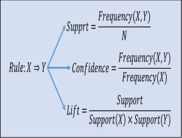
Items that occur more frequently in transactions are more important than others; and rules based on frequently occurring itemsets have better predictive power. Support and Confidence are two measures based on frequency of itemsets that are used to build association rules.
| transaction ID | milk | bread | butter | beer | diapers |
|---|---|---|---|---|---|
| 1 | 1 | 1 | 0 | 0 | 0 |
| 2 | 0 | 0 | 1 | 0 | 0 |
| 3 | 0 | 0 | 0 | 1 | 1 |
| 4 | 1 | 1 | 1 | 0 | 0 |
| 5 | 0 | 1 | 0 | 0 | 0 |
Support
Support is an indication of how frequently the itemset apppears in the database

Total number of transaction = 5
Number of times itemset {beer, diapers} appears = 1
Support of {beer, diapers} = 1/5 = 0.2
Confidence
It is an indication of how often the rule has be found to be true

supp(XUY) is support of union of items in X and Y.
For rule {butter, bread} ==> {milk}
supp(XUY) = support of {butter, bread, milk} = 1/5 = 0.2
supp(X) = support of {butter,bread} = 1/5 = 0.2
confidence of the rule = 0.2/0.2 = 1
Thus indicating that the rule is correct, and that 100% of times when customer buys bread and butter, milk is bought as well.
Lift
It indicates how likely is the RHS itemset to be picked along with LHS itemset than by itself

supp(XUY) is support of union of items in X and Y
For rule {milk, bread} ==> {butter}
supp(XUY) = support of {milk, bread, butter} = 1/5 = 0.2
supp(X) = suppport of {milk,bread} = 2/5 = 0.4
supp(Y) = support of {butter} = 2/5 = 0.4
lift of rule = 0.2/0.4*0.4 = 1.25
If lift = 1, it would imply that the probability of occurrence of the antecedent and that of the consequent are independent of each other.
When two events are independent of each other no rule can be drawn involving those two events.
If lift > 1, that lets us know the degree to which two occurrences are dependent on one another and makes those rules potentially useful for predicting the consequent in future data sets.
What is the challenge in AR?
Finding all frequent itemsets in a database is difficult since it involves searching all possible item combinations. For n number of items, the possible itemsets are 2^n - 1, it is called power-set and excludes empty sets. The size of the power-set grows exponentially in the number of items n so to make the search more efficient downward-closure method is used by algorithms which guarantees that for a frequent itemset, all its subsets are also frequent and thus no infrequent itemset can be a subset of a frequent itemset.
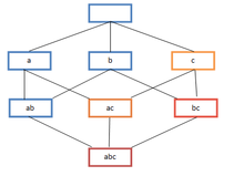
Frequent itemset lattice, where the color of the box indicates how many transactions contain the combination of items. Note that lower levels of the lattice can contain at most the minimum number of their parents' items; e.g. {ac} can have only at most min(a,c). This is called the downward-closure propertys.
Algorithms like Apriori take user-specified minimum support and minimum confidence as input to build rules:
- minimum support threshold is applied to find all frequent itemsets in a database
- minimum support confidence constraint is applied to these frequent itemsets in order to form rules
How Apriori AR algorithm gets frequent items?
See the video below for a step by step tutorial on how to run apriori algorithm to get the frequent item sets.

Download the groceries data
Groceries data is available in arules package or you can find it at below url - download and save as groceries.csv
https://raw.githubusercontent.com/stedy/
Machine-Learning-with-R-datasets/master/groceries.csv
Build the sparse matrix for transactions data
Groceries transaction data is not structured - people buy different items. To give it structure all possible items as are stored as columns and transactions as rows with values 1 for items bought in the transaction and 0 for remaining items.
If there are thousands of items and millions of transactions, the rows will have many zeros for items not bought in the individual transaction - this is sparse data. In R we read in such data as transactions so that they are stored in sparse matrix in which the zero values are not recorded - they are empty cells. This makes sparse matrix more memory efficient compared to data frames.
# install and load the R packages for association rules
install.packages("arules")
library(arules)
# see the datasets available in package arules
data(package="arules")
Data sets in package ‘arules’:
Adult Adult Data Set
AdultUCI Adult Data Set
Epub Epub Data Set
Groceries Groceries Data Set
Income Income Data Set
IncomeESL Income Data Set
class(Groceries)
[1] "transactions"
attr(,"package")
[1] "arules"
head(Groceries)
transactions in sparse format with
6 transactions (rows) and
169 items (columns)
# if groceries data is be stored in external file as csv
# we read them in as transactions
Groc = read.transactions("<path>/groceries.csv", sep=",")
Groc
transactions in sparse format with
9835 transactions (rows) and
169 items (columns)
Inspect Transactions
Here we inspect the transactions
Note: we use inspect function instead of just subsetting the itemMatrix for Groceries data Groc
# inspect first three transactions
inspect(Groc[1:3])
items
1 {citrus fruit,
margarine,
ready soups,
semi-finished bread}
2 {coffee,
tropical fruit,
yogurt}
3 {whole milk}
# to see frequency/support of item 1
itemFrequency(Groc[,1])
abrasive cleaner
0.003558719
# Actual number of times item 1 occurred is
0.003558719*9835
[1] 35
# to see frequency/support of first 6 items
itemFrequency(Groc[ ,1:6])
abrasive cleaner artif. sweetener baby cosmetics baby food bags
0.0035587189 0.0032536858 0.0006100661 0.0001016777 0.0004067107
baking powder
0.0176919166
# to see frequency/support of items 1 to 8
itemFrequency(Groc[ ,1:8])
abrasive cleaner artif. sweetener baby cosmetics baby food
0.0035587189 0.0032536858 0.0006100661 0.0001016777
bags baking powder bathroom cleaner beef
0.0004067107 0.0176919166 0.0027452974 0.0524656838
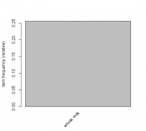
Plot items for given minimum Support
# plot all items with specified min support
itemFrequencyPlot(Groc, support=0.20)
#shows only whole milk
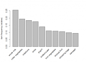
# reduce support to 10 percent
itemFrequencyPlot(Groc, support=0.1)
#shows below items
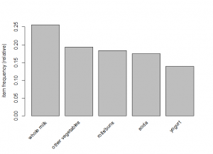
#plot items with top 5 support
itemFrequencyPlot(Groc, topN=5)
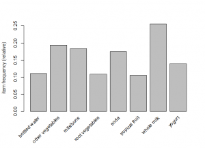
#plot items with top 10 support
itemFrequencyPlot(Groc, topN=10)
Apriori Algorithm to select association rules
High confidence implies rule has good predictive accuracy. Apriori algorithm first identifies high support itemsets, then high confidence association rules for those itemsets.
# use apriori function in the arules package
?apriori
apriori {arules} R Documentation
Mining Associations with Apriori
Description
Mine frequent itemsets, association rules or association
hyperedges using the Apriori algorithm.
The Apriori algorithm employs level-wise search for
frequent itemsets. The implementation of Apriori used
includes some improvements (e.g., a prefix tree and item sorting).
Usage
apriori(data, parameter = NULL, appearance = NULL, control = NULL)
parameter
object of class APparameter or named list.
The default behavior is to mine rules with support 0.1,
confidence 0.8, and maxlen 10
Examples:
data("Adult")
Mine association rules.
rules <- apriori(Adult,
parameter = list(supp = 0.5, conf = 0.9, target = "rules"))
summary(rules)
# use apriori on groceries to get rules with atleast 2 items
# and support 0.007 and confidence 25 percent
assoc_rule = apriori(Groc, parameter=list(
support=0.007,
confidence=0.25,
minlen=2))
Parameter specification:
confidence minval smax arem aval originalSupport support minlen maxlen
0.25 0.1 1 none FALSE TRUE 0.007 2 10
target ext
rules FALSE
Algorithmic control:
filter tree heap memopt load sort verbose
0.1 TRUE TRUE FALSE TRUE 2 TRUE
apriori - find association rules with the apriori algorithm
version 4.21 (2004.05.09) (c) 1996-2004 Christian Borgelt
set item appearances ...[0 item(s)] done [0.00s].
set transactions ...[169 item(s), 9835 transaction(s)] done [0.01s].
sorting and recoding items ... [104 item(s)] done [0.00s].
creating transaction tree ... done [0.00s].
checking subsets of size 1 2 3 4 done [0.00s].
writing ... [363 rule(s)] done [0.00s].
creating S4 object ... done [0.00s].
# see the number of rules identified by rules
assoc_rule
set of 363 rules
#see the summary of algorithm
summary(assoc_rule)
set of 363 rules
rule length distribution (lhs + rhs):sizes
2 3 4
137 214 12
Min. 1st Qu. Median Mean 3rd Qu. Max.
2.000 2.000 3.000 2.656 3.000 4.000
support confidence lift
Min. :0.007016 Min. :0.2500 Min. :0.9932
1st Qu.:0.008134 1st Qu.:0.2962 1st Qu.:1.6060
Median :0.009659 Median :0.3551 Median :1.9086
Mean :0.012945 Mean :0.3743 Mean :2.0072
3rd Qu.:0.013777 3rd Qu.:0.4420 3rd Qu.:2.3289
Max. :0.074835 Max. :0.6389 Max. :3.9565
mining info:
data ntransactions support confidence
Groc 9835 0.007 0.25
class(assoc_rule)
[1] "rules"
attr(,"package")
[1] "arules"