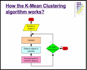
K-Means Clustering Algorithm
How it Works?
By Victor Lavrenko

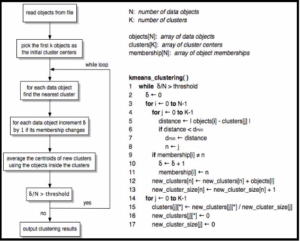
Programming Logic
Steps to cluster data points based on numerical features using KMeans clustering algorithm and compare the results with Hierarchical clustering.
Pre-requisite:
Understand the dataset for pre-processing that may be requierd for clustering algorithm.
Step 1:
Remove the categorical variable from the dataset.
Step 2:
Use k-means function for number of clusters.
Step 3:
Scatter plot two dimensions colour coding data points per the k-means cluster members. Also plot the cluster centers and interpret the plot.
Step 4:
Compare the cluster members with actual values of the categorical variable.
Step 5:
Now use Hierarchical clustering and plot Dendogram
Step 6:
Interpret Dendogram ad compare the with k-means scatter plot for cluster members.
Data pre-processing
We remove the categorical variable 'Species' from the dataset and use remaining four to identify the clusters using k-means clustering.
# now we remove the 'Species' column from the data
# this is to make sure the data is unlabeled
iris_numerical =iris[,-5]
str(iris_numerical)
#'data.frame': 150 obs. of 4 variables:
# $ Sepal.Length: num 5.1 4.9 4.7 4.6 5 5.4 4.6 5 4.4 4.9 ...
# $ Sepal.Width : num 3.5 3 3.2 3.1 3.6 3.9 3.4 3.4 2.9 3.1 ...
# $ Petal.Length: num 1.4 1.4 1.3 1.5 1.4 1.7 1.4 1.5 1.4 1.5 ...
# $ Petal.Width : num 0.2 0.2 0.2 0.2 0.2 0.4 0.3 0.2 0.2 0.1 ...
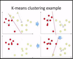
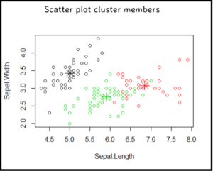
Scatter plot
Plot two dimensions colour coding the data points based on which KMeans cluster they belong to; and show the cluster centers.
# there are four dimensions to the data but we use only two
# plot Sepal length & width and colour as per cluster
# membership
plot(iris_numerical[c("Sepal.Length","Sepal.Width")],
col = kmeansClustering$cluster)
#plot cluster centers for the clusters
points(kmeansClustering$centers[,c("Sepal.Length", "Sepal.Width")], col =1:3, pch=8, cex=2)
Interpret cluster members scatter plot
Some red points are closer to the green center, this is due to remaining two dimensions viz. Petal.Length and Petal.Width which are not included in the scatter plot.
Compare with actual values
Lets compare the cluster members with the actual total values for the categorical attribute.
#Lets compare the kmeans cluster with the Species classes
table(iris$Species, kmeansClustering$cluster)
# 1 2 3
# setosa 50 0 0
# versicolor 0 48 2
# virginica 0 14 36
# cluster setosa can be separated from other clusters
# clusters versicolor and virginica have a small degree of overlap
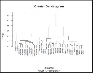
Plot Dendogram
See the Hierarchical clusters using dendogram.
# plot dendogram for hierarchical clustering
plot(iris_numerical_40_hc)
# plot(iris_numerical_40_hc, hang=-1, labels=iris$Species[index])
plot(iris_numerical_40_hc,
labels=iris$Species[index],
cex=0.6)
Interpret cluster member dendogram
Similar to k-means cluster here also we can see that setosa can be separated from remaining two clusters, clusters virginca and versicolor are overlapping