Type I Error & Type II Error
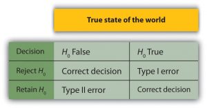
When null is true:
Type I Error is rejecting the null when it is true (probability = α)
Correct decision is not rejecting the null when it is true (probability = 1- α)
When null is false:
Type II Error is failing to reject the null when it is false (probability = β)
Correct decision is rejecting the null when it is false (probability = 1- β)
Example: Study to see effect of two medicines to treat patients
To see the effect of two medicines the null hypothesis is the default statement that there is no difference between the medicines. To validate this statement null hypothesis testing is done on a sample data of the population. There are two datasets representing two samples for the effect of two medicines and the test statistic means is used.
Null Hypothesis: The two medicines have same effect, that is, the means of two samples are equal.
Null Hypothesis Testing: (H0): μ1= μ2
Alternate Hypothesis: The two medicines have different effect, that is, the means of two samples are not equal.
Alternate Hypothesis Testing: (H1): μ1≠ μ2
Type I error occurs when the study rejects the null hypothesis and concludes that the two medicines are different when actually they have the same effect.
Consequence of Type I error: Rejecting a medicine as less effective is not that big a problem because patients have at least one medicine for treatment.
Type II error occurs when the study fails to reject the null hypothesis and concludes that both the medicines are effective in treating the patients when actually one of them is not.
Consequence of Type II error: Not rejecting a medicine that can not treat patients can cost patients their life as such this error is not acceptable.
Evaluating the Risk of Type I error and Type II error
Depending on which error costs more the level of tolerance called significance is set while testing the null hypothesis using a particular statistic.
P-value ( p )
Probability Value is the probability of the statistic used to test the null hypothesis. p-value along with probability of occurrence of type I and type II errors determines whether to reject or not reject the null hypothesis.
Significance ( α )
Is the acceptable level of Type I error denoted as α. Say a 5 percent of tolerance is allowed for Type I error beyond which the null hypothesis is rejected. That is out of 20 samples, we're willing to accept one rejection of null hypothesis even if it is true. α can also be 1 percent if consequences of Type I error are costly.
If p-value < α - that is less than tolerance of Type I error - then the null hypothesis is rejected in favor of the alternate hypothesis.
Power of Test ( 1-β )
Similarly, the acceptable level of Type II error is denoted as β. β is probability of not rejecting null hypothesis when it is false; so (1-β) is correctly rejecting the null hypothesis when it is false and hence it is called the power of the statistical test.
Typically level of acceptance for type I error α is 5 percent; generally the target for β is 20 percent or 10 percent thus 80 percent or 90 percent is set as the target for power of test.
Interpreting the statistical test result:
α = 0.05
p = 0.04
Since p < α we reject the null hypothesis.
This however, does not mean that there is 4 % probability that null hypothesis is true. It means that assuming null hypothesis is true, the sample data exhibits the statistical test with probability 0.04.
It is conditional probability P(D/H0) = 0.04
D - the event that sample data exhibits the test statistic
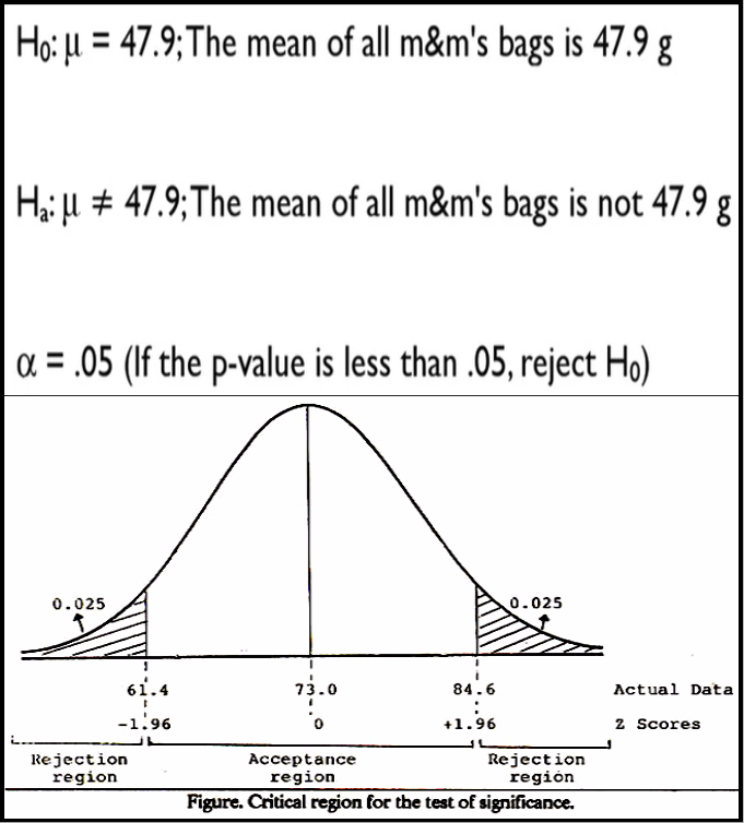
Critical Region
If the test statistic falls in this region under the normal distribution curve of the sample data the null hypothesis is rejected.
This region is depicted as the extreme value on either the left, right or both sides of the normal curve, that is near the tail.
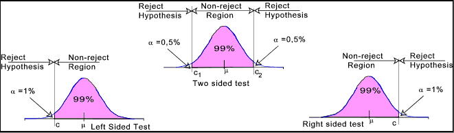
One-Tailed Null Hypothesis Testing
When the critical region ( i.e. null hypothesis rejection region ) is only one side of the normal distribution curve - either left tail or right tail it is called one-tailed null hypothesis.
It is also called directional hypothesis testing because the alternate hypothesis rejects the null hypothesis by comparing the test statistic value to be either greater than or less than the reference value specified in the null hypothesis.
For example:
H0: μ = 20 vs. H1: μ > 20
H0: μ = 200 vs. H1: μ < 300
Two-tailed Null Hypothesis Testing
When the critical region ( i.e. null hypothesis rejection region ) is on both sides of the normal distribution curve - left and right tail it is called two-tailed null hypothesis testing.
It is also called non-directional hypothesis testing because the alternate hypothesis rejects the null hypothesis if the test statistic value is not equal to the reference value specified in the null hypothesis - regardless of whether it is greater than or less than the specified value.
For example:
H0: μ = 850 vs. H1: μ≠ 850
One-Sample t.test
Understanding the Lung Capacity dataset
We load the tab separated data file which has the Lung Capacity dataset.
# load lung capacity data
# from text file with tab delimited columns
lungCapacity_df = read.csv("~/dataFiles/LungCapData.txt", header=T, sep="\t")
class(lungCapacity_df)
# [1] "data.frame"
# see the rows and columns in data frame
dim(lungCapacity_df)
# [1] 725 6
str(lungCapacity_df)
# 'data.frame': 725 obs. of 6 variables:
# $ LungCap : num 6.47 10.12 9.55 11.12 4.8 ...
# $ Age : int 6 18 16 14 5 11 8 11 15 11 ...
# $ Height : num 62.1 74.7 69.7 71 56.9 58.7 63.3 70.4 70.5 59.2 ...
# $ Smoke : Factor w/ 2 levels "no","yes": 1 2 1 1 1 1 1 1 1 1 ...
# $ Gender : Factor w/ 2 levels "female","male": 2 1 1 2 2 1 2 2 2 2 ...
# $ Caesarean: Factor w/ 2 levels "no","yes": 1 1 2 1 1 1 2 1 1 1 ...
names(lungCapacity_df)
# [1] "LungCap" "Age" "Height" "Smoke" "Gender" "Caesarean"
# see summary of lung capacity
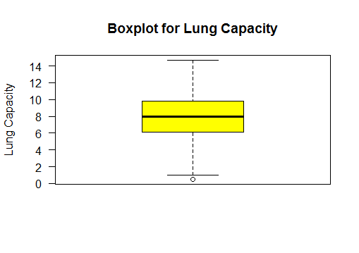
summary(lungCapacity_df$LungCap)
# Min. 1st Qu. Median Mean 3rd Qu. Max.
# 0.507 6.150 8.000 7.863 9.800 14.680
Boxplot Lung Capacity
#boxplot lung capacity
boxplot(lungCapacity_df$LungCap,
col=c("yellow"),
main="Boxplot for Lung Capacity",
ylab="Lung Capacity", las=1)
Interpret the t.test result
Here test statistic is based on single statistic. For example mean of Lung Capacity for the given dataset.
Null Hypothesis: Mean of LungCap is greater than 8
H0: μ >= 8 vs. H1: μ < 8
# we test with 5 percent significance level
# that is, confidence interval 95 %
Test.one.sided.95 = t.test(lungCapacity_df$LungCap,
mu=8,
alt="less",
conf=0.95)
Test.one.sided.95
# One Sample t-test
# data: lungCapacity_df$LungCap
# t = -1.3842, df = 724, p-value = 0.08336
# alternative hypothesis: true mean is less than 8
# 95 percent confidence interval:
# -Inf 8.025974
# sample estimates:
# mean of x
# 7.863148
names(Test.one.sided.95)
# [1] "statistic" "parameter" "p.value" "conf.int" "estimate"
# [6] "null.value" "alternative" "method" "data.name"
# to reject or not to reject the null hypothesis
p = Test.one.sided.95$p.value
significance = 0.05
Result = ifelse( (p - significance)>0,
"NULL is True",
"Alternate is True: Reject Null" )
Result
# [1] "NULL is True"
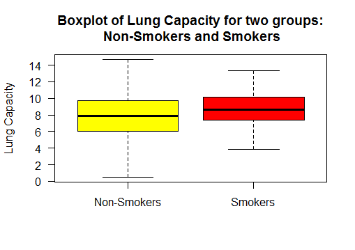
Boxplot the two sample populations
Group 1 : Lung Capacity of Non-Smokers
Group 2 : Lung Capacity of Smokers
It shows the lung capacity of non-smokers has higher variance than that of smokers.
# lung capacity for smokers and non-smokers
class(lungCapacity_df$LungCap)
#[1] "numeric"
class(lungCapacity_df$Smoke)
#[1] "factor"
summary(lungCapacity_df$LungCap)
# Min. 1st Qu. Median Mean 3rd Qu. Max.
# 0.507 6.150 8.000 7.863 9.800 14.680
summary(lungCapacity_df$Smoke)
# no yes
# 648 77
# box plot lungcapacity wrt to smoker - yes or no
boxplot(lungCapacity_df$LungCap~lungCapacity_df$Smoke)
Paired t-test
Here the t-test is done on two populations that are dependent on each other.
We use the blood pressure dataset which records the blood pressure of patients before and after treatment.
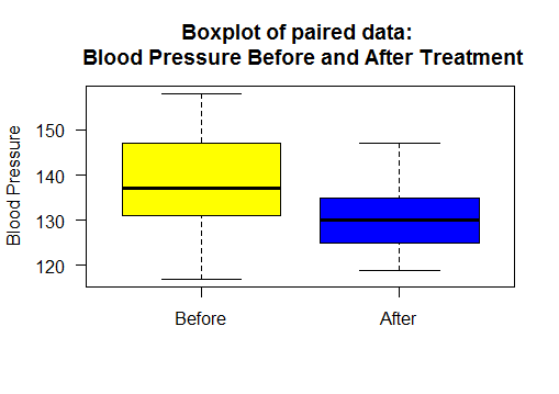
Blood pressure before and after treatment
We compare the means of below two dependent populations:
μ1 - mean of blood pressure before treatment
μ2 - mean of blood pressure after treatment
Null Hypothesis: Two means are equal
Alternate Hypothesis : Two means are not equal, two-tailed testing
H0: μ1 = μ2 vs. H1: μ1 ≠ μ2
Boxplot and Scatter Plot for paired dataset
Boxplot of blood pressure before and after treatment.
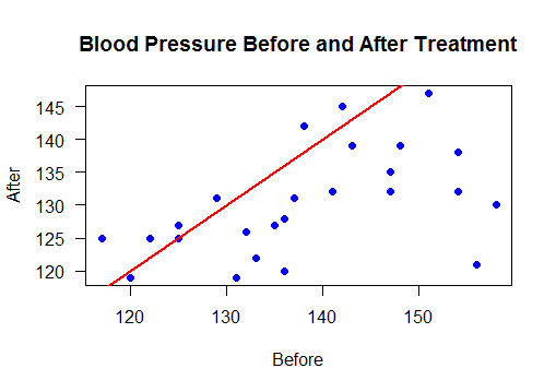
Scatter plot with regression line
Points below the line show reduced blood pressure after treatement
#boxplot
boxplot(bloodPressure$Before, bloodPressure$After,
names=c("Before","After"),
col=c("yellow","blue"),
main="Boxplot of paired data: \n Blood Pressure Before and After Treatment",
ylab="Blood Pressure", las=1)
#Scatter plot
plot(bloodPressure$Before, bloodPressure$After,
main="Blood Pressure Before and After Treatment",
xlab="Before", ylab="After",las=1,pch=19, col="blue")
abline(a=0, b=1, col="red",lwd=2)