Linear Regression 

Supervised Learning

Regression problem is one that predicts a continuous value based on previously known inputs. Input values are called predictors and output is called response. Here we predict or estimate an actual value not a class as in classification.

lr-formula

lr-slope

lr-slope-expl

Our regression problem

In this example we fit a linear regression model for relationship between scalar dependent variable cpi (customer price index for each quarter) and independent variable quarter.

We have previous known data for cpi for each quarter of three years 2012 to 2014. We use the model to predict cpi for quarters of the year 2015.

# consumer price index (cpi)
# quarterly cpi for three years

cpi = c(162.2, 164.6, 166.5, 166.2,
167.0, 168.6, 169.5, 171.0,
171.0, 172.1, 173.3, 174.0)

# each year has four quarters

year = rep(2012:2014, each=4)
year
# [1] 2012 2012 2012 2012 2013 2013 2013 2013 2014 2014 2014 2014

# and four quarters for each of three years

quarter = rep(1:4,3)
quarter

Programming Logic

Steps to fit the linear regression model for relationship between dependent and independent variables.

Step 1:
Find the correlation between dependent variable cpi and independent variables year and quarter

Step 2:
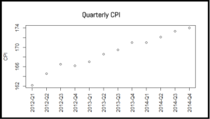
Scatter plot dependent vs independent variables

Step 3:
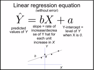
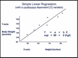
Fit the linear regression model and determine the coefficients

Step 3:
Using the model predict the cpi for each quarter of year 2015

Step 4:
Plot the cpi for previous years and for the predicted year


Correlation between variables


cor(year,cpi)
# [1] 0.9076727

cor(quarter,cpi)
# [1] 0.3968641

Plot to visualize the correlation

cpi-yr-qtr


# cpi~ year + quarter

# plot cpi vs quarter to see the relationship
# plot cpi for each quarter for three years
# define x axis manually using axis function

plot(cpi, xaxt="n", ylab="CPI", xlab="")
axis(1, labels=paste(year, quarter, sep="-Q"), at=1:12, las=3)

Fit the linear regression model


# cpi ~ year + quarter

lrm = lm(cpi ~ year + quarter)

print(lrm)
# Call:
# lm(formula = y ~ x, data = data_new)

# Coefficients:
# (Intercept)          x
#   9.743                1.509

Predict using linear regression model


# predict cpi for each quarter of year 2015

data2015 = data.frame(year=2015, quarter=1:4)
cpi2015 = predict(lrm, newdata = data2015)
cpi2015
# 1                   2                 3                 4
# 174.7083   175.9417   177.1750    178.4083

Plot the previous and predicted values

cpi-predicted


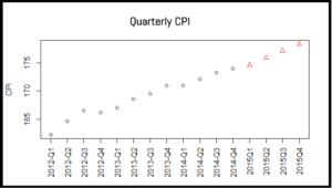
# now plot the predicted values and previous values

# there are 16 values, last four are predicted so use different style for last four
# repeat style 1, 12 times and repeat 2 four times

style = c(rep(1,12), rep(2,4))
plot(c(cpi,cpi2015), xaxt="n", ylab="CPI", xlab="", pch=style, col=style)
axis(1,labels=c(paste(year,quarter,sep="Q"),
"2015Q1","2015Q2","2015Q3","2015Q4"),at=1:16,las=3)