Polynomial Regression
Supervised Learning
.
.
Regression problem is one that predicts a continuous value based on previously known inputs. Input values are called predictors and output is called response. Here we predict or estimate an actual value not a class as in classification.
.
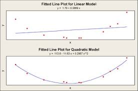
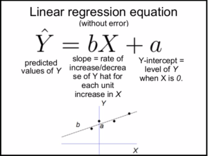
Regression measures the contribution of the independent variables to the variability of dependent variable. Simple linear regression uses formula with predictors raised to the power of 1 (a linear combination of monomials) and a straight line is fitted to depict the relationship.
.
Simple linear regression is a good fit if the relationship is highly correlated; however, in many cases it may not be so and a curve may explain the relationship better. Polynomial regression helps capture such relationship by extending linear regression formula - it uses predictors raised to the power of 2, 3, 4 and so on until adding higher polynomials does not further explain the variability of the dependent variable significantly compared to the previous.
Names of polynomials by degree:
- Degree 0 – constant
- Degree 1 – linear
- Degree 2 – quadratic
- Degree 3 – cubic
- Degree 4 – quartic (or, if all terms have even degree, biquadratic)
- Degree 5 – quintic
and so on... See Polynomials : Wikipedia
How far do we go?
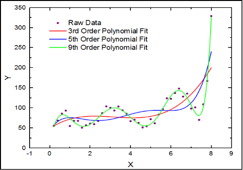
In simple linear regression we face the problem of under-fitting whereas in polynomial regression, if we go on adding the degree of polynomials we could be over-fitting by explaining the noise along with the signal and thus making the model unsuitable for prediction. So in most practical scenarios we do not fit beyond cubic polynomials.
.
Linear_model = lm(y ~ x)
Quadratic_model = lm(y ~ x + x^2)
Cubic_model = lm(y ~ x + x^2 + x^3)
Programming Logic
Steps to fit the simple linear & polynomial regression models to compare the influence of independent variables on the response variable.
Step 1:
Find the correlation between dependent variable dist and independent variable speed
Step 2:
Scatter plot dependent vs independent variables to see if there is any pattern in the distribution
Step 3:
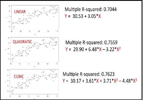
Fit the linear regression model, note the significance and multiple r-squared value
Step 4:
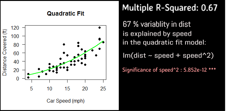
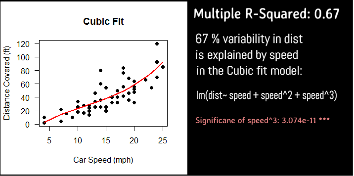
Fit the quadratic and cubic polynomial regression models and note the significance and multiple r-squared value
Step 5:
Plot the lines for predicted values of response using the linear, quadratic and cubic regression models
Step 6:
Do the analysis of vairance for the linear, quadratic and cubic models to decide which is the best fit for prediction.
Plot to visualize the correlation
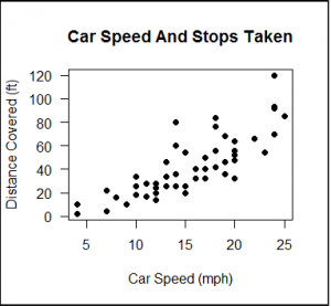
#scatter plot dist~speed
# pch=19 is solid circle
plot(cars$dist~cars$speed, pch=19,
xlab="Car Speed (mph)",
ylab="Distance Covered (ft)",
main = "Car Speed And Stops Taken",
las=1)
Fit the quadratic polynomial regression model
# now fit quadratic polynomial model
fitQ = lm(dist~poly(speed,2,raw=TRUE), data=cars)
#analysis of variance
anova(fitQ)
# Analysis of Variance Table
# Response: dist
# Df Sum Sq Mean Sq F value Pr(>F)
# poly(speed, 2, raw = TRUE) 2 21714 10857.1 47.141 5.852e-12 ***
# Residuals 47 10825 230.3
# ---
# Signif. codes: 0 ‘***’ 0.001 ‘**’ 0.01 ‘*’ 0.05 ‘.’ 0.1 ‘ ’ 1
#summary to get the r-squared value
summary(fitQ)
# Call:
# lm(formula = dist ~ poly(speed, 2, raw = TRUE), data = cars)
# Residuals:
# Min 1Q Median 3Q Max
# -28.720 -9.184 -3.188 4.628 45.152
# Coefficients:
# Estimate Std. Error t value Pr(>|t|)
# (Intercept) 2.47014 14.81716 0.167 0.868
# poly(speed, 2, raw = TRUE)1 0.91329 2.03422 0.449 0.656
# poly(speed, 2, raw = TRUE)2 0.09996 0.06597 1.515 0.136
# Residual standard error: 15.18 on 47 degrees of freedom
# Multiple R-squared: 0.6673, Adjusted R-squared: 0.6532
# F-statistic: 47.14 on 2 and 47 DF, p-value: 5.852e-12
# R-squared is 0.67, that 67 percent variability is due to predictors
# Residual Error is 15.18
Plot the predicted values using the three regression models
Linear
Quadratic
Cubic
#plot the prediction using the linear model
plot(cars$dist~cars$speed, pch=19,
xlab="Car Speed (mph)",
ylab="Distance Covered (ft)",
main = "Linear Fit",
las=1)
#draw the linear regression fit line
lines(cars$speed, predict(fitlm), col="blue", lwd=2)
#plot the prediction using the quadratic model
plot(cars$dist~cars$speed, pch=19,
xlab="Car Speed (mph)",
ylab="Distance Covered (ft)",
main = "Quadratic Fit",
las=1)
#draw the quadratic regression fit line
lines(cars$speed, predict(fitQ), col="green", lwd=2)
#plot the prediction using the cubic model
plot(cars$dist~cars$speed, pch=19,
xlab="Car Speed (mph)",
ylab="Distance Covered (ft)",
main = "Cubic Fit",
las=1)
#draw the cubic regression fit line
lines(cars$speed, predict(fitC), col="red", lwd=2)
Compare the three regression models:
Linear
Quadratic
Cubic
Linear Vs Quadratic Vs Cubic
Which regression model do we select?
As compared to the Linear model, Quadratic model explains the variability more significantly and also the curvature is a better fit than the straight line..
Adding the cubic term does not improve the significance greatly as compared to quadratic term of the predictor, speed, so there is no added advantage to using it.
So we prefer quadratic over cubic and linear models.
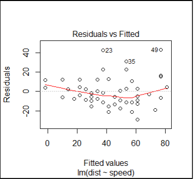
#plot the residuals for linear model
plot(fitlm,which=1)
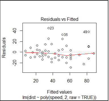
#plot the residuals for quadratic model
plot(fitQ,which=1)