Grid World Model-Free Optimal Policy

Model-free Reinforcement Learning

In reinforcement learning(RL), a model-free algorithm (as opposed to a model-based one) is an algorithm which does not use the transition probability distribution(and the reward function) associated with the Markov decision process (MDP), which, in RL, represents the problem to be solved.

The transition probability distribution (or transition model) and the reward function are often collectively called the "model" of the environment (or MDP), hence the name "model-free".

A model-free RL algorithm can be thought of as an "explicit" trial-and-error algorithm. An example of a model-free algorithm is Q-learning.

Wikipedia: Model-free RL

Solving 2x2 Grid World MDP

We will use the Reinforcement Learning R package to implement the model-free solution through dynamic learning from interactive interactions of the agent with the environment.

Programming Steps:

1. Define environment function that mimics the environment

2. Create Sample Experience

3. Learning Phase

4. Evaluate the policy

5. Summary of RL model

6. Apply a policy to unseen data

7. Update the existing policy with new observational data

8. Evaluate updated RL model

9. Plot the reward for learning iterations

10. Conclusion

2by2GridStates

RL-reward-iteration-plot

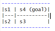
2x2 Grid MDP

(Source: Reinforcement Learning in R, by Nicolas Pröllochs, Stefan Feuerriegel)

Here we using the Reinforcement Learning Package to find the optimal solution for the grid problem. We have no information about the transition probabilities hence it is the model-free approach.

2by2GridStates

Reinforcement Learning Environment

The robot is in an environment, two-by-two grid and will take some actions and will move into a new state and or will receive a reward for moving to that state.
We're going to observe the agent interacting with the environment over and over and over again

we're going to observe which of the possible actions the agent randomly takes
what is the reward the agent receives
the reward is a signal of how well the agent is performing
our goal is that we want to improve behaviour

Given this limited feedback reward signal, we want to find the optimal policy for moving from state to state to maximise rewards.

Install & load R ReinforcementLearning package

#Install using devtools

install.packages("devtools")

# Download and install latest version from Github

devtools::install_github("nproellochs/ReinforcementLearning")

# Load the package

library(ReinforcementLearning)
library(dplyr)

Environment Description:

The inbuilt gridworldEnvironment function simulates the environment for the agent to learn from.

# Load the exemplary environment (gridworld)

?gridworldEnvironment

Description

Function defines an environment for a 2x2 gridworld example.

Here an agent is intended to navigate from an arbitrary starting position to a goal position.
The grid is surrounded by a wall, which makes it impossible for the agent to move off the grid. In addition, the agent faces a wall between s1 and s4.
If the agent reaches the goal position, it earns a reward of 10.
Crossing each square of the grid results in a negative reward of -1.

Usage

gridworldEnvironment(state, action)

Define environment function that mimics the environment

We pass the state-action pairs to the environment function which then returns the next state and the reward. For the grid mdp, we have an inbuilt function in the Reinforcement Learning package.

You can see the function models the environment:

every possible action the agent can take
what the new state will be
and every possible reward the agent will receive for moving from state to state

#Note: to copy function code call without ()

env = gridworldEnvironment
print(env)

## function (state, action) 
## {
##     next_state <- state
##     if (state == state("s1") && action == "down") 
##         next_state <- state("s2")
##     if (state == state("s2") && action == "up") 
##         next_state <- state("s1")
##     if (state == state("s2") && action == "right") 
##         next_state <- state("s3")
##     if (state == state("s3") && action == "left") 
##         next_state <- state("s2")
##     if (state == state("s3") && action == "up") 
##         next_state <- state("s4")
##     if (next_state == state("s4") && state != state("s4")) {
##         reward <- 10
##     }
##     else {
##         reward <- -1
##     }
##     out <- list(NextState = next_state, Reward = reward)
##     return(out)
## }
## <bytecode: 0x00000000109e4718>
## <environment: namespace:ReinforcementLearning>

Define state and action sets

states = c("s1", "s2", "s3", "s4")
states

## [1] "s1" "s2" "s3" "s4"

actions = c("up", "down", "left", "right")
actions

## [1] "up"    "down"  "left"  "right"

Create Sample Experience

To learn the agent we need a random sample of interactions of the agent with the environment for the given mdp - this is called the sample experience that is used for simulation during the actual learning process. For this, we pass the sample size, states, actions and environment objects to the inbuilt sampleExperience function which returns the data object comprising the random sequence of experienced state transition tuples (si, ai, ri+1, si+1) for the given sample size.

# See the sampleExperience function

?sampleExperience

Description

Function generates sample experience in the form of state transition tuples.

Usage

sampleExperience(N, env, states, actions, actionSelection = "random",
control = list(alpha = 0.1, gamma = 0.1, epsilon = 0.1), model = NULL,
...)

Arguments

N - Number of samples.
env - An environment function.
states - A character vector defining the enviroment states.
actions - A character vector defining the available actions.
actionSelection (optional) - Defines the action selection mode of the reinforcement learning agent. Default: random.
control (optional) - Control parameters defining the behavior of the agent. Default: alpha = 0.1; gamma = 0.1; epsilon = 0.1.
model (optional) Existing model of class rl. Default: NULL.
...
Additional parameters passed to function.
Value

A dataframe containing the experienced state transition tuples s,a,r,s_new. The individual columns are as follows:

State
The current state.

Action
The selected action for the current state.

Reward
The reward in the current state.

NextState
The next state.

Define the data for sample experience

Create the data for the simulation using the sampleExperience function and passing the sample size, states, actions as input.

For simulation, we have to create a sample run for N times.

Let's sample the agent's behaviour a thousand times, Sample N = 1000, random sequences from the environment

# Data format must be (s, a,r,s_new) tuples as rows in a data frame

data = sampleExperience(N = 1000,
                        env = env,
                        states = states,
                        actions = actions)

head(data)

##   State Action Reward NextState
## 1    s3  right     -1        s3
## 2    s1     up     -1        s1
## 3    s1     up     -1        s1
## 4    s3     up     10        s4
## 5    s2   left     -1        s2
## 6    s1   down     -1        s2

dim(data)

## [1] 1000    4

#Let's examine a subset of the data

s4_data = data %>% 
          filter(NextState == state("s4"))

dim(s4_data)

## [1] 315   4

head(s4_data)

##   State Action Reward NextState
## 1    s3     up     10        s4
## 2    s4   down     -1        s4
## 3    s3     up     10        s4
## 4    s4  right     -1        s4
## 5    s4     up     -1        s4
## 6    s4   down     -1        s4

Learning Phase Control Parameters

For this, we call the ReinforcementLearning function passing the sampleExperience object as input along with the control parameters like learning rate, discount factor and the exploration greediness value. It returns the rl object.

alpha - the learning rate, set between 0 and 1.

gamma - discount, discounts the value of future rewards and weigh less heavily

epsilon - the balance between exploration and exploitation

# RL control paramters

control = list(alpha = 0.1,
               gamma = 0.5,
               epsilon = 0.1)

control

## $alpha
## [1] 0.1
## 
## $gamma
## [1] 0.5
## 
## $epsilon
## [1] 0.1

Perform Reinforcement Learning

Model-free reinforcement learning requires input data in the form of sample sequences consisting of states, actions and rewards. The result of the learning process is a state-action table and an optimal policy that defines the best possible action in each state.

Usage

ReinforcementLearning(data, s = “s”, a = “a”, r = “r”, s_new = “s_new”, learningRule = “experienceReplay”, iter = 1, control = list(alpha = 0.1, gamma = 0.1, epsilon = 0.1), verbose = F, model = NULL, …)

# Build the Reinforcement Learning Model

model = ReinforcementLearning(
                data, 
                s = "State",
                a = "Action",
                r = "Reward",
                s_new = "NextState",
                control = control)

print(model)

## State-Action function Q
##        right         up       down       left
## s1 -0.662419 -0.6590728  0.7644642 -0.6559966
## s2  3.573507 -0.6527449  0.7611561  0.7377884
## s3  3.587911  9.1349318  3.5744963  0.7749757
## s4 -1.872785 -1.8205106 -1.8582109 -1.8644346
## 
## Policy
##      s1      s2      s3      s4 
##  "down" "right"    "up"    "up" 
## 
## Reward (last iteration)
## [1] -285

Evaluate the policy

The policy function takes the rl object and returns the best possible action in each state. This is the optimal policy the agent has learned. If we print the rl object we get the state-action pairs, Q-value of each state-action pair.

For state s1 best action is down - it has the highest reward 0.76

For state s2 best action is right - it has the highest reward 3.58

For state s3 best action is up - it has the highest reward 9.13

For state s4 best action is left - it has the highest reward -1.87

And that is indicated by the best policy.

print(gridWold_RL_model)

## State-Action function Q

##        right         up       down       left
## s1 -0.662419 -0.6590728  0.7644642 -0.6559966
## s2  3.573507 -0.6527449  0.7611561  0.7377884
## s3  3.587911  9.1349318  3.5744963  0.7749757
## s4 -1.872785 -1.8205106 -1.8582109 -1.8644346
## 
## Policy
##      s1      s2      s3      s4 
##  "down" "right"    "up"    "up" 
## 
## Reward (last iteration)
## [1] -285

Summary of RL model

The summary function outputs the diagnostics regarding the model such as the number of states, actions and distribution of cumulative reward.

If the total reward is highly negative it indicates that the random policy used to generate the state transition samples deviates from the optimal case and hence the need to apply & update a learned policy with new data samples.

# Print summary statistics

summary(model)

#>
#> Model details
#> Learning rule: experienceReplay
#> Learning iterations: 1
#> Number of states: 4
#> Number of actions: 4
#> Total Reward: -340
#>
#> Reward details (per iteration)
#> Min: -340
#> Max: -340
#> Average: -340
#> Median: -340
#> Standard deviation: NA

Apply a policy to unseen data

To evaluate the out-of-sample performance of the agent for the existing policy we pass unseen data, states, and use the model to predict the best action for those states.

# Example data
data_unseen = 
       data.frame(State = c("s1", "s2", "s3"),
                   stringsAsFactors = FALSE)

#Pick optiomal action
data_unseen$OptimalAction = 
            predict(model, data_unseen$State)

data_unseen
'
 State OptimalAction
1 s1 down
2 s2 right
3 s3 up
'

Update the existing policy with new observational data

This is beneficial when new data points become available or when one wants to plot the reward as a function for different training samples. Here we pass additional input parameter, RL model, to the sampleExperience function to get the random sample for reinforcement learning. Specifying actionSeclection mode as 'epsilon-greedy' instead of default mode random, thereby following the best action with probability 1 - ε and a random one with ε.

# Sample N = 1000 sequences from environment 
# using epsilon-greedy action selection 

data_new = sampleExperience(N = 1000, 
             env = env, 
             states = states, 
             actions = actions, 
             actionSelection = "epsilon-greedy", 
             model = model, 
             control = control) 

" {compare to the previous sampleExperience  
       data = sampleExperience(N = 1000,  
           env = env,  
           states = states,  
           actions = actions) } "


# Update existing policy using new training data
model_new = ReinforcementLearning(data_new,
                       s = "State",
                       a = "Action",
                       r = "Reward",
                s_new = "NextState",
                  control = control,
                      model = model)


"
{
compare it to previous model

model = ReinforcementLearning(data,
                       s = 'State',
                      a = 'Action',
                      r = 'Reward',
               s_new = 'NextState',
                 control = control)

}

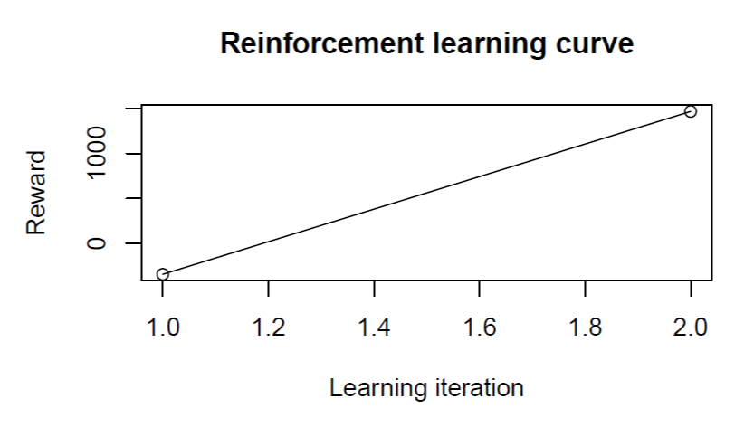
Evaluate updated RL model

The following code snippet shows that the updated policy yields
significantly higher rewards as compared to the previous policy.
These changes can also be visualized in a learning curve via plot
(model_new).

# Print result
print(model_new)

'
State-Action function Q
 right up down left
s1 -0.6386208 -0.6409566 0.7640001 -0.6324682
s2 3.5278760 -0.6384522 0.7624763 0.7710285
s3 3.5528350 9.0556251 3.5632348 0.7672169
s4 -1.9159520 -1.9443706 -1.9005900 -1.8888277

Policy
 s1 s2 s3 s4 
 "down" "right" "up" "left" 

Reward (last iteration)
[1] 1277

Plot RL Curve

Plot the cumulative reward for the learning iterations.

# Plot reinforcement learning curve
plot(model_new)