Hierarchical Clustering

Clustering

Unsupervised Learning

Cluster analysis or clustering is the task of grouping a set of objects in such a way that objects in the same group (called a cluster) are more similar (in some sense or another) to each other than to those in other groups (clusters)

scatter-plot-simple

hc-cl-1

hc-numbers-1

How is Clustering different than Classification and Regression ?

Clustering is classification without saying which classes observations have to belong to or how many classes there are. There is no need for training data, the clustering algorithm identifies the clusters.

No prior knowledge is required of the result

No training data available.

No labels

No right or wrong, plenty possible clusterings

Programming Logic

Steps for analysing the given dataset using clustering algorithms

Pre-requisite:

Understand the dataset for any pre-processing that may be required

Step 1:
Scatter plot two dimensions of dataset and interpret the plots

Step 2:
Data pre-processing and scaling using normalization

Step 3:
Calculate Euclidean distance for the companies w.r.t to each other

Step 4:
Identify clusters of companies using Hierarchical clustering methods complete linkage and average linkage.

Step 5:
Plot Dendograms for Hierarchical clusters and interpret the plots

Step 6:
Compare the cluster membership using the two methods of Hierarchical clustering

Step 7:
Interpret the cluster-wise statistics

Understanding data set

We read a csv file containg the data for our cluster analysis.

There are 22 observations of 9 variables.

Company is the one categorical variable others are all numerical data variables. Hierarchical clustering is used to identify clusters based on the numerical variables and assign members, in this case variable 'company' to a cluster based on similarities w.r.t. to these variables.

#read csv file

utilities = read.csv("C:/utilities.csv")

dim(utilities)
# [1] 22 9

str(utilities)
# 'data.frame': 22 obs. of 9 variables:
# $ Company : Factor w/ 22 levels "Arizona","Boston",..: 1 2 3 4 5 6 7 8 9 10 ...
# $ Fixed_charge: num 1.06 0.89 1.43 1.02 1.49 1.32 1.22 1.1 1.34 1.12 ...
# $ RoR : num 9.2 10.3 15.4 11.2 8.8 13.5 12.2 9.2 13 12.4 ...
# $ Cost : int 151 202 113 168 192 111 175 245 168 197 ...
# $ Load : num 54.4 57.9 53 56 51.2 60 67.6 57 60.4 53 ...
# $ D.Demand : num 1.6 2.2 3.4 0.3 1 -2.2 2.2 3.3 7.2 2.7 ...
# $ Sales : int 9077 5088 9212 6423 3300 11127 7642 13082 8406 6455 ...
# $ Nuclear : num 0 25.3 0 34.3 15.6 22.5 0 0 0 39.2 ...
# $ Fuel_Cost : num 0.628 1.555 1.058 0.7 2.044 ...

Scatter plot the data set

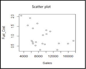
To identify the clusters w.r.t Fuel_cost and Sales, we scatter plot data points using these two dimensions.

#Scatter Plot two variables Fuel_Cost and Sales

plot(Fuel_Cost~Sales, utilities)

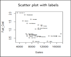
# add names next to the scatter dots

with(utilities, text(Fuel_Cost~Sales, labels=Company))

# the names and dots overlap, so lets add position to labels, pos=1 is at bottom, size of text is cex value

with(utilities, text(Fuel_Cost~Sales, labels=Company, pos=4, cex=0.4))

Interpret the scatter plot

Left side companies have high fuel_cost and low sales. In the middle companies have medium sales and medium fuel_cost. Right side low fuel cost and high sales.

So based on these two variables we have broadly identified three clusters

scatter-plot-simple

scatter-plot-labels

Data pre-processing for clustering

# we consider only quantitative data so remove 'Company' from analysis

utilities_new = utilities[,-1]
str(utilities_new)

# 'data.frame': 22 obs. of 8 variables:
# $ Fixed_charge: num 1.06 0.89 1.43 1.02 1.49 1.32 1.22 1.1 1.34 # 1.12 ...
# $ RoR : num 9.2 10.3 15.4 11.2 8.8 13.5 12.2 9.2 13 12.4 ...
# $ Cost : int 151 202 113 168 192 111 175 245 168 197 ...
# $ Load : num 54.4 57.9 53 56 51.2 60 67.6 57 60.4 53 ...
# $ D.Demand : num 1.6 2.2 3.4 0.3 1 -2.2 2.2 3.3 7.2 2.7 ...
# $ Sales : int 9077 5088 9212 6423 3300 11127 7642 13082 8406 6455 ...
# $ Nuclear : num 0 25.3 0 34.3 15.6 22.5 0 0 0 39.2 ...
# $ Fuel_Cost : num 0.628 1.555 1.058 0.7 2.044 ...

Scaling data using normalization

When we normalize the variables, average for each variable becomes zero and standard deviation approximately 1 .

We use apply in R as below:

#apply(X, MARGIN, FUN, optional args to function)

# get mean of columns i.e. margin 2 of data set

means = apply(utilities_new,2,mean)
str(means)
#Named num [1:8] 1.11 10.74 168.18 56.98 3.24 ...
# - attr(*, "names")= chr [1:8] "Fixed_charge" "RoR" "Cost" "Load" ...
means
# Fixed_charge RoR Cost Load D.Demand Sales
# 1.114091 10.736364 168.181818 56.977273 3.240909 8943.000000
# Nuclear Fuel_Cost
# 13.868182 0.962000

# get standard deviation of columns i.e. margin 2 of data set

sdev = apply(utilities_new,2,sd)
str(sdev)
# Named num [1:8] 0.185 2.244 41.191 4.461 3.118 ...
# - attr(*, "names")= chr [1:8] "Fixed_charge" "RoR" "Cost" "Load" ...
sdev

# Fixed_charge RoR Cost Load D.Demand Sales
# 0.1845112 2.2440494 41.1913495 4.4611478 3.1182503 3533.1966505

# Nuclear Fuel_Cost
# 17.6572766 0.4997877

length(means)
[1] 8

length(sdev)
[1] 8

length(utilities_new)
[1] 8

# now use the scale function to normalize

utilities_norm = scale(utilities_new, means, sdev)
str(utilities_norm)
# num [1:22, 1:8] -0.293 -1.215 1.712 -0.51 2.037 ...
# - attr(*, "dimnames")=List of 2
# ..$ : NULL
# ..$ : chr [1:8] "Fixed_charge" "RoR" "Cost" "Load" ...
# - attr(*, "scaled:center")= Named num [1:8] 1.11 10.74 168.18 56.98 3.24 ...
# ..- attr(*, "names")= chr [1:8] "Fixed_charge" "RoR" "Cost" "Load" ...
# - attr(*, "scaled:scale")= Named num [1:8] 0.185 2.244 41.191 4.461 3.118 ...
# ..- attr(*, "names")= chr [1:8] "Fixed_charge" "RoR" "Cost" "Load" ...

head(utilities_norm)

# Fixed_charge RoR Cost Load D.Demand Sales
# [1,] -0.2931579 -0.6846390 -0.417122002 -0.5777152 -0.52622751 0.03792600
# [2,] -1.2145113 -0.1944537 0.821002037 0.2068363 -0.33381191 -1.09107994
# [3,] 1.7121407 2.0782236 -1.339645796 -0.8915357 0.05101929 0.07613502
# [4,] -0.5099470 0.2066070 -0.004413989 -0.2190631 -0.94312798 -0.71323514
# [5,] 2.0373243 -0.8628882 0.578232617 -1.2950193 -0.71864311 -1.59713726
# [6,] 1.1159709 1.2315399 -1.388199680 0.6775672 -1.74485965 0.61813712
# Nuclear Fuel_Cost
# [1,] -0.78540888 -0.6682838
# [2,] 0.64742817 1.1865039
# [3,] -0.78540888 0.1920816
# [4,] 1.15713304 -0.5242226
# [5,] 0.09807958 2.1649194
# [6,] 0.48885332 0.5582371

Calculate Euclidean Distance

Euclidean distances or Euclidean metric is the straight distance between two points in Euclidean space.

It shows the distance between the rows of data matrix for a column, for example, cell(11,7) is 6.05 which indicates that 11 th company and 7 th company are very dissimilar and that for cell(13,10) it is 1.40 which indicates 13 th company and 10 th company are very similar.

# calculate Euclidean distance

distance = dist(utilities_norm)
distance
print(distance, digits=3)

# 1 2 3 4 5 6 7 8 9 10 11 12 13 14 15
# 2 3.17
# 3 3.70 4.92
# 4 2.38 2.28 4.07
# 5 4.30 3.87 4.55 4.28
# 6 3.62 4.23 2.97 3.23 4.66
# 7 4.00 3.42 4.25 4.01 4.60 3.35
# 8 2.75 4.02 5.04 3.66 5.37 4.96 4.52
# 9 3.29 4.48 3.11 3.77 5.26 4.09 3.61 3.46
# 10 3.01 2.81 3.89 1.49 4.21 3.86 4.54 3.62 3.53
# 11 3.50 4.83 5.91 4.83 6.56 6.01 6.05 3.49 5.26 5.04
# 12 2.29 2.79 3.78 2.69 4.40 3.65 2.39 3.03 2.21 3.14 4.81
# 13 3.85 3.52 4.31 2.56 4.90 4.57 5.02 4.04 3.52 1.40 5.24 3.68
# 14 2.11 4.38 2.77 3.17 4.98 3.49 5.00 4.34 3.83 3.54 4.32 3.66 4.29
# 15 2.68 2.46 5.17 3.19 4.28 4.05 2.94 3.97 4.56 4.26 4.78 2.49 5.08 4.30
# 16 4.04 4.89 5.28 4.93 5.95 5.85 5.13 2.22 3.66 4.48 3.43 4.03 4.32 5.17 5.23
# 17 4.54 3.62 6.40 4.99 5.63 6.12 4.58 5.61 5.55 5.57 4.87 4.19 5.69 5.68 3.43
# 18 1.92 2.90 2.72 2.60 4.41 2.83 2.99 3.31 2.87 3.02 3.96 2.12 # 3.70 2.35 3.01
# 19 2.41 4.69 3.20 3.41 5.28 2.60 4.61 4.12 4.14 4.07 4.53 3.80 4.93 1.88 4.09
# 20 3.08 3.08 3.67 1.81 4.52 2.93 3.56 4.04 2.94 2.06 5.31 2.57 2.23 3.67 3.76
# 21 3.16 2.45 5.29 2.15 4.70 4.36 3.93 3.27 3.85 2.54 4.74 2.70 2.76 4.68 3.15
# 22 2.53 2.44 4.09 2.63 3.83 4.03 3.98 3.32 3.66 2.62 3.44 2.96 2.79 3.53 3.32

# 16 17 18 19 20 21
# 2
# 3
# 4
# 5
# 6
# 7
# 8
# 9
# 10
# 11
# 12
# 13
# 14
# 15
# 16
# 17 5.68
# 18 4.00 4.48
# 19 5.23 6.19 2.51
# 20 4.77 4.95 2.85 3.83
# 21 4.27 4.33 3.55 4.74 2.17
# 22 3.48 3.65 2.51 3.98 2.66 2.50

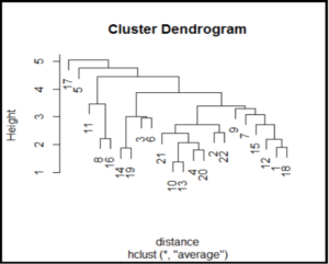
Hierarchical Clustering

Use hclust clustering function which uses Complete Linkage as default method. For Average Linkage specify the method.

# Hierarchical cluster using default Complete Linkage

hCluster.cl = hclust(distance)

print(hCluster.cl)

# Call:
# hclust(d = distance)

# Cluster method : complete
# Distance : euclidean
# Number of objects: 22

# Hierarchical cluster using default Complete Linkage

hCluster.al = hclust(distance, method="average")

print(hCluster.al)

# Call:
# hclust(d = distance, method = "average")

# Cluster method : average
# Distance : euclidean
# Number of objects: 22

Plot Dendogram

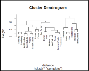
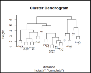
For Hierarchical clustering using both methods, complete linkage and average linkage plot dendograms with company name as labels.

# Dendogram

plot(hCluster.cl, labels=utilities$Company, cex=0.6)

Interpret Dendograms

Hierarchical Clustering Complete Linkage

Company 10 and Company 13 are most closely related

hc-numbers-1

hc-cl-1

Hierarchical Clustering Average Linkage

Company 10 and Company 13 are most closely related

hc-al-numbers-1

hc-cl-1

Cluster membership

Hierarchical clustering assigns members to same cluster depending on similarities. For simplicity we retrieve members of first three clusters.

# cluster membership for three clusters

member.cl = cutree(hCluster.cl, 3)
member.al = cutree(hCluster.al,3)

Compare Hierarchical Cluster Methods

We see which companies are assigned to which cluster using complete linkage vs average linkage methods for first three clusters.

15 companies are members of cluster 1 by both methods
2 companies that are members of cluster 1 by average linkage belong to cluster 2 by complete linkage methods and so on

# use confusion matrix for membership of both the methods

table(member.cl, member.al)

# member.al
# member.cl 1 2 3
# 1 15 1 0
# 2 2 0 1
# 3 3 0 0

Cluster-wise statistics

Using aggregate function we can find the mean of each feature for members of each cluster.

For cluster 3 Sales is highest and Fuel_cost is lowest whereas for companies in cluster 2 Sales is low with highest Fuel_cost.

# cluster-wise statistics

aggregate(utilities_norm, list(member.cl), mean)

# Group.1 Fixed_charge RoR Cost Load
# 1 1 0.2488147 0.3235831 -0.2062161 0.2008503
# 2 2 -0.7267360 -0.8925964 -0.2390911 1.5517816
# 3 3 -0.6002757 -0.8331800 1.3389101 -0.4805802

# D.Demand Sales Nuclear Fuel_Cost
# 1 -0.2135522 -0.2243011 0.2619639 -0.1121726
# 2 0.1472271 -0.6608746 -0.6117317 1.3912575
# 3 0.9917178 1.8571473 -0.7854089 -0.7930034

# instead of taking normalized values you can also look at the original values

aggregate(utilities_new, list(member.cl), mean)

# Group.1 Fixed_charge RoR Cost Load
# 1 1 1.160000 11.462500 159.6875 56.08125
# 2 2 0.980000 8.733333 158.3333 63.90000
# 3 3 1.003333 8.866667 223.3333 54.83333

# D.Demand Sales Nuclear Fuel_Cost
# 1 2.575000 8150.50 18.493750 0.9059375
# 2 3.700000 6608.00 3.066667 1.6573333
# 3 6.333333 15504.67 0.000000 0.5656667